XI. General Character of Ocean Currents
The theory of ocean currents will be presented in chapters XII, XIII, and XIV. Here the currents will be discussed nonmathematically, partly as an introduction to the more exact treatment, and partly to facilitate a study of the chapter on water masses and currents of the oceans for those who are not completely familiar with the theories of hydrodynamics. The ocean currents may be conveniently divided into three groups: (1) currents that are related to the distribution of density in the sea, (2) currents that are caused directly by the stress that the wind exerts on the sea surface, and (3) tidal currents and currents associated with internal waves.
To the first class belong the well-known large-scale currents of the oceans, such as the Gulf Stream, the Kuroshio, the Equatorial Currents, the Benguela Current, and others. All of these currents transport great amounts of waters. Their courses at the surface are known from ships' observations (p. 428), and at subsurface depths their character has, in a few localities, been derived from direct measurements of currents from anchored vessels, and in many more localities they have been ascertained from determinations of temperatures and salinities. The methods used for drawing conclusions as to currents from such observations will be discussed below.
The wind drift transports water in one and the same direction over large areas if it blows prevailingly from one direction, but the currents that are associated with tides and internal waves run alternatingly in opposite direction or are rotating. Although tidal currents may attain high velocities, they are of no direct importance to the circulation of the ocean waters.
Currents Related to the Distribution of Density. An explanation of the nature of the currents that are related to the distribution of density in the sea can be based upon a few simple laws of physics. One of these states that the acceleration of a body equals the sum of the forces that act per unit mass of the body. This law, which is applicable to any part of a fluid, implies that, if a body moves with a uniform velocity, the forces that act on the body balance each other. Another law of physics states that within a fluid a force is exerted in the direction
In the oceans the pressure increases downward, and the pressure gradient that is directed against decreasing pressure is therefore directed upward. It is so nearly vertical that it practically balances the acceleration of gravity per unit mass. If it exactly balanced the acceleration of gravity, the isobaric surfaces would coincide with the level surfaces and perfect static equilibrium would exist. Actually, the isobaric surfaces in the ocean slope slightly relative to the level surfaces, but the slope is so small that quasi-static equilibrium exists, meaning that along any vertical the distance between two isobaric surfaces can be found if the density of the water in the interval is known. Let the pressure at the two isobaric surfaces be p1 and p2, respectively, and let the average density along a vertical be  . The corresponding vertical distance between the isobaric surfaces is then h = (p1 − p2)/g
 , where g is the acceleration of gravity. Therefore the distance is great where the average density of the water is small, and vice versa.
The small deviations from a state of perfect static equilibrium can be found if the density of the water at different depths is known with great accuracy. From these deviations—that is, from the slopes of the isobaric surfaces—conclusions can be drawn as to the ocean currents, taking the acting forces into account. Along an isobaric surface the pressure gradient is, by definition, zero, and consequently no force related to the distribution of pressure acts along such a surface. If an isobaric surface coincides with a level surface, no component of gravity acts along the surface, and if the water is at rest it will remain at rest. On the other hand, if an isobaric surface slopes relative to a level surface, a component of gravity acts along it, and the water cannot remain at rest. It must move down the sloping surface, but as soon as it is set in motion the effect of the earth's rotation has to be considered.
In order to describe conveniently and precisely the motion of any moving mass on the earth, it is necessary to introduce the deflecting force of the earth's rotation (Corioli's force), which is proportional to the speed at which the mass moves and is directed at right angles to the velocity—to the right in the Northern Hemisphere and to the left in the Southern. The reason for introducing this force is explained on p. 432. Corioli's force is so weak that in nearly all problems of mechanics it can be neglected, because other acting forces are so much greater, but when dealing with the atmosphere and the oceans the weak Corioli's force becomes highly significant, because other forces are small.
With regard to the motion of the water, it can be stated that this motion is no longer accelerated if the component of gravity acting along the isobaric surface is balanced by Corioli's force. The component of gravity is directed down-slope, and Corioli's force must therefore be directed up-slope. Since Corioli's force is directed at right angles to the current, the current follows the contours of the sloping isobaric surface. In the Northern Hemisphere the isobaric surface slopes upward to the right of an observer looking in the direction of the current; in the Southern Hemisphere it slopes upward to the left.
The numerical value of the velocity for a given slope is
In middle latitudes even the strongest surface currents rarely have velocities above 100 cm/sec (about 2 knots). In latitude 45° the corresponding slope of the sea surface is 1.05 × 10⁻⁵; that is, the surface drops or rises about 1 cm in 105 cm (1 km), or about 1 m in 105 m (100 km). Such a gentle slope cannot possibly be observed directly, but the slope of one isobaric surface relative to another can be determined if the density of the water at two neighboring localities is accurately known at a number of depths. The sea surface can always be considered an isobaric surface, and the slope of the sea surface relative to an isobaric surface at any depth below the surface can be determined from the density distribution. If at two neighboring stations A and B the average density between the sea surface and, say, 1000 m is less at A than at B, the distance between an isobaric surface at a depth of about 1000 m and the sea surface, is greater at A than it is at B. Relative to the isobaric surface at about 1000 m, the sea surface slopes downward from A to B. If this relative slope is to be determined with sufficient accuracy, the density must be known to the fifth decimal place, meaning that errors in salinity determinations must not exceed 0.02 ‰ and errors in temperature observations must not exceed 0.02°C. This is one reason for the many efforts to improve the accuracy of salinity and temperature measurements.
From relative slopes relative currents can be computed, but we wish to determine absolute currents. It is therefore necessary to find the absolute slopes of the isobaric surfaces, and valid conclusions as to absolute slope can often be drawn from a careful examination of the vertical and horizontal distribution of temperature and salinity or from consideration
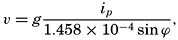
The computations needed for constructing such topographic charts are commonly called dynamic computations. In these computations a vertical distance is expressed by means of the work that is performed or gained in moving a unit mass from one level to another. The work is expressed in the unit dynamic meter, which represents the work performed in lifting a unit mass nearly 1 m. When dynamic meters are used, charts of geopotential (dynamic) topography of isobaric surfaces are prepared. The contours represent lines along which a body can be moved without work having to be performed against gravity, and, if the contours are drawn at equal intervals of dynamic distance, the same work is always performed or gained in moving a unit mass from one contour to another. Within a small area, no perceptible difference exists between the contours expressed in units of dynamic meters or ordinary meters, but over large areas the two types of contours do not coincide, because the acceleration of gravity varies with latitude. The velocity of the current in meters per second is obtained by the formula
From a chart of the topography of an isobaric surface the corresponding currents are readily obtained on the assumptions that have been made, namely, that the component of gravity acting along the isobaric surface is balanced by Corioli's force. On this assumption the current is directed along the contours. If these are drawn at equal intervals, the slope of the surface is inversely proportional to the horizontal distance
Charts of currents which are constructed in this manner give pictures that are only approximately correct. In the first place, errors may have been introduced by the selection of a reference isobaric surface. These errors are difficult to avoid, because such selection requires not only thorough familiarity with oceanographic data and with the principles of hydrodynamics, but also a certain amount of judgment. In the second place, errors are introduced because the distribution of density changes in the course of time, the implication being that the velocity of any moving water mass is always changing; that is, that accelerations which have been neglected are not quite absent. It can be shown, however, that the velocities computed by neglecting accelerations are rarely more than a few per cent in error (p. 453). More serious are the errors which may be introduced by treating the oceanographic observations as if they were simultaneous. It has been tacitly assumed that simultaneous observations were available from a number of localities, but in general the data to be used have been obtained on a cruise of a single vessel, and the occupation of the stations may have taken weeks or months. For each individual area it is desirable to determine the time interval within which work must be completed in order to avoid serious distortion of the picture of the currents. It can be stated in general, however, that the closer the stations are spaced the shorter must be the period in which they are occupied and that ocean-wide currents can be examined by means of stations which are far apart and which have been occupied in different years and seasons.
In the third place, frictional forces have been neglected. This omission is not a serious matter, because, according to accumulated experience, the influence of friction on currents that are related to the distribution of density is small.
In the fourth place, it has been assumed that the slopes of the isobaric surfaces depend entirely upon the distribution of density and that, in general, one level isobaric surface can be found to which all slopes can be referred. This assumption is not always true. The surface of no motion may slope so much that it does not coincide with any isobaric surface, but the difficulty here is only minor. Within a small region the surface of no motion can be considered level, and by proceeding step by step one can find the slope of the sea surface or of any other isobaric surface relative to the layer of no motion. A more serious difficulty arises when the slope of the sea surface is caused not only by the water masses having different densities, but also by actual piling up of water in some localities and removal of water in others. In landlocked bodies of water, such as the Baltic or the Gulf of Bothnia, piling up of water by wind may lead
So many reservations have been made that it may appear as if the computed currents have little or no relation to the actual currents. Fortunately, however, most of the assumptions made lead only to minor errors, and currents can be correctly represented in the first approximation by means of the slopes of a series of isobaric surfaces relative to one reference surface. In the Straits of Florida an excellent agreement has been obtained between observed and computed currents (fig. 184, p. 674); off the Grand Banks of Newfoundland the computed currents have been used successfully by the International Ice Patrol for predicting the drift of icebergs (p. 668); and in many areas results of computations have been checked against directly observed surface currents or results of drift-bottle experiments. The method that has been outlined has therefore become standard procedure in physical oceanography.
It was stated that in the Northern Hemisphere the current is so directed that the isobaric surfaces slope upward to the right of an observer looking in the direction of flow and that the distances between isobaric surfaces increase with decreasing density. Provided that the level of no motion lies at some distance below the sea surface, one has then the simple rule: In the Northern Hemisphere the lighter water lies on the right-hand side of an observer looking in the direction of the current, and the denser water lies on the left hand. In the Southern Hemisphere the lighter water lies to the left and the denser water to the right.
Inasmuch as the density of the water near the surface is generally more dependent on the temperature than on the salinity, the term “lighter” may be replaced by “warmer,” and “denser” by “colder.” These rules greatly facilitate a rapid survey of the directions of the currents if charts are available showing the distribution of density or of temperature at different depths below the surface or in vertical sections. In general, the distribution of density is represented by σt or by anomalies of specific volume, δ (pp. 56–59).
Greater differences in density in a horizontal direction are found only in the upper layers of the ocean, and hence steep relative slopes of isobaric surfaces are present in the upper layers only. If the deeper and more uniform water masses are moving slowly, it follows that steep absolute slopes and corresponding swift currents are limited to the upper layers. In some areas the currents that are related to the distribution of density are negligible at a depth of 500 m or less (California Current, Equatorial Countercurrents), in others at 1000 or 2000 m (Kuroshio, Gulf Stream),
In general, the flow of the deep water cannot be computed from the distribution of density, mainly because in the deep water the differences in density in a horizontal direction are so small that they cannot as yet be determined with sufficient accuracy. Conclusions as to the motion of the deep water are therefore based directly upon an examination of the distribution of temperature and salinity, and not upon the computations that have been outlined.
The transport of water by the currents can be obtained from the computed velocities or directly from the distribution of density. Computation of transport is often useful for determining a layer of no motion, because the amount of water that is transported into any ocean region must nearly equal the amount that is transported out of the region in the same time. The difference must equal the difference between evaporation on one hand and precipitation and runoff from land on the other hand. This difference is, in general, small compared to the water masses that are transported by currents. Similarly, the net amount of salt carried by currents into any ocean region must be zero, a fact that may be used independently or in conjunction with consideration of the transport of water (p. 457).
In the preceding discussion, no mention has been made of cause and effect. The reason is that any given distribution of density can remain unaltered in course of time only in the presence of currents of the type that has been described. Therefore, all that can be stated is that a mutual relation exists between the distribution of density and the corresponding currents, but it is impossible to tell whether the distribution of density causes the currents or the currents cause the distribution of density. In order to enter upon the causal relationship, it is necessary to consider the factors that influence the distribution of density—namely, the processes of heating and cooling and the effect of the wind. The heating and cooling were discussed in chapter IV, and here emphasis will be placed on the effect of the wind.
Wind Currents and the Secondary Effect of the Wind Toward Producing Ocean Currents. The effect of the wind on the ocean currents is twofold. In the first place, the stress that the wind exerts on the sea surface leads directly to the development of a shallow wind drift; in the second place, the transport of water by the wind drift leads to an altered distribution of density and the development of corresponding currents.
In the case of the wind drift, only frictional forces and Corioli's forces are important. The wind exerts a stress on the sea surface which
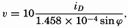
It follows that a depth can always be found at which the current flows in a direction exactly opposite to that of the surface current. At this depth the velocity has decreased, on the assumption of a constant eddy viscosity, to a small fraction of its value at the surface, and below this depth the currents are negligible. Ekman therefore calls this depth the depth of frictional resistance. The thickness of the layer above the depth of frictional resistance can roughly be considered equal to the thickness of the layer which under the influence of prevailing winds is stirred up so thoroughly that it is nearly homogeneous. The depth of frictional resistance increases with increasing wind velocity and with decreasing latitude. At the Equator it is theoretically infinite. The relations between depth of frictional resistance, D, wind velocity, W, and latitude, ϕ, are expressed approximately by 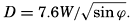 . The depth is obtained in meters when the wind velocity is given in meters per second. Similarly, at the sea surface the velocity of the wind drift is approximately
 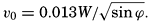 .
.
The total transport due to the wind drift is directed at right angles to the wind, in the Northern Hemisphere to the right and in the Southern Hemisphere to the left. This transport is independent of the character and the numerical value of the eddy viscosity and depends only upon the stress of the wind and the latitude.
The wind drift that has been described can develop only in the open ocean in regions where the wind blows in the same direction and with the same velocity over wide areas. Near coasts and near regions of wind shifts, modifications arise and the secondary effect of the wind becomes important. Consider a wind which in the Northern Hemisphere blows parallel to a coast that is on the right-hand side of an observer
If the coast lies to the left of the wind direction, the light and warm surface water is transported away from the coast and is replaced by denser and colder subsurface water. This process, which is known as upwelling, also leads to an altered distribution of density to which a current flowing in the direction of the wind corresponds. Experience shows that the upwelling is restricted to shallow depths, and its effect can be traced only to depths of 100 to 300 m. The phenomenon of upwelling has been studied extensively, partly because the cold subsurface water that is drawn up to the surface exercises a great influence upon the climates of the coasts where upwelling occurs, and partly because the upwelling water is rich in plant nutrients. Regions of upwelling are therefore regions of high productivity. These relations are dealt with elsewhere, and here it needs only to be emphasized that the upwelling is a direct effect of the wind and that, as a secondary effect, a current develops parallel to the coast and in the direction of the wind.
In the open ocean, analogous conditions are encountered. Where an atmospheric anticyclone is located over the ocean, the prevailing winds tend to transport the light surface water toward the center of the anticyclone. Owing to this transport, an accumulation of light water is maintained near the center of the anticyclone, and corresponding to this distribution of density a current must be present that again flows in the direction of the wind.
From this discussion it is clear that the prevailing winds are of primary importance to the current systems of the oceans. This importance is seen by a comparison of charts showing the prevailing winds and currents, because in many regions the directions closely coincide. There are notable exceptions, however, which are mainly caused by the necessity of the coastal currents to follow the coast lines.
It would be wrong, however, to place too great emphasis on the importance of the winds in maintaining the ocean currents, because in homogeneous water an entirely different system would develop. The
Tidal Currents. In contrast to currents that are related to the distribution of density or to the wind, tidal currents do not bring about a transport of water over large distances. In sounds and narrow straits the tidal currents reverse their direction every six hours where a semidiurnal tide dominates and every twelve hours where a diurnal tide is present. In the open ocean the tidal currents are, in general, rotating, owing to the effect of Corioli's force; that is, from hour to hour the currents change in both direction and velocity. In the Northern Hemisphere the change in direction is clockwise; in the Southern Hemisphere it is counterclockwise. The current completes one rotation in about twelve hours where the tide is semidiurnal and in about twenty-four hours where the tide is diurnal. The net transport of water in twelve or twenty-four hours is therefore zero. Theoretically, the tidal currents should run in the same direction and with the same velocity from the surface to the bottom except in the lowest 20 to 30 m, where they are influenced by bottom friction. The correctness of this conclusion has been verified in shallow waters, but observations sufficient for verification are not available from the deep sea.
The tidal currents vary from one locality to another, depending upon the character of the tide, the depth to the bottom, and the configuration of the coast, but in any given locality they repeat themselves as regularly as the tides to which they are related. In the open ocean, however, they are less readily observed because they are superimposed upon other currents that vary in an irregular manner and that can be eliminated only when long series of observations are available. Information as to tidal currents has primarily been collected from regions in which these currents are of importance to navigation.
From the point of view of the marine biologist the most important aspect of the tidal currents is that they contribute greatly toward the stirring of the water layers, particularly in coastal areas, where the currents can attain velocities up to several knots.
Currents that are related to internal waves are in general of tidal period, but these currents vary in direction and velocity with depth. In the open ocean they can attain much higher velocities than the tidal
The tidal currents are maintained by rhythmic variations in the slopes of the isobaric surface. The rise and fall of the tide, which is caused by the action of the moon and the sun, demonstrates that water is rhythmically piled up (high water) or removed (low water). The sea surface slopes down from a region of high water to one of low water, and all isobaric surfaces below the sea surface slope similarly, but six hours later the direction of the down-slope is reversed. The water particles therefore move under the influence of a periodically varying force, and the corresponding motion is an oscillation comparable to the oscillation of a pendulum, except that Corioli's force makes the particles move in ellipses instead of back and forth along a straight line, where such elliptic orbits are not prevented by boundaries.
Internal waves can be considered as being maintained by rhythmic variations in the distribution of density, which, according to the relation between the distributions of density and pressure, is equivalent to rhythmic variation in the slopes of the isobaric surfaces. In an internal wave, one or more isobaric surfaces at intermediate depth remain level, however, and the slopes of the isobaric surfaces above or below a level surface are in opposite directions. The corresponding currents are also in opposite directions, and, if several internal waves of different periods are present simultaneously, a complicated pattern of currents is found.
From this brief summary it is evident that it is virtually impossible to obtain knowledge of the ocean currents on an entirely empirical basis. If this were to be accomplished, it would be necessary to conduct measurements from anchored vessels at numerous localities for long periods and at many depths. By means of such measurements the different types of periodic currents could be examined, and by averaging they could be eliminated and the other types studied. In many oceanographic problems, however, knowledge of the periodic current is less essential. The currents that transport water over long distances are the important ones. Currents related to the distribution of density can be computed from the more easily observed temperatures and salinities, following the procedure which has been outlined here and which will be discussed in detail in the following chapters, and wind currents can be examined theoretically. Herein lies the value of the application of hydrodynamics to oceanography and the necessity of familiarity with this application if all possible conclusions shall be drawn from the observed distributions.