Appendix:
Restating the Bargaining Model

In this appendix, we reconstruct more rigorously our bargaining model by further appropriating concepts from the corpus of micro-economic theory. We continue to concentrate on the variables time and impatience and reciprocal demand intensity through indifference analysis. Recall that an indifference curve represents various combinations of quantities of rewards X and Y (e.g., revenue and basic resources) among which an entity is indifferent, or is equally satisfied. In Figure 9, A's indifference curves are arrayed in an indifference map—a series of indifference curves. Each curve is convex to the zero intercept,

. On the map the curves move farther to the right and farther from the zero intercept. Each curve lying farther to the right reflects relatively more preferred positions. Entity B's

[43] René Dumont with Marcel Mazoyer, Socialisms and Development (New York: Praeger, 1973), p. 335.

[44] See the report of a speech by Tanzania's minister for agriculture, Joseph Mungai, to a conference of the Inter-Africa Coffee Organization in Dar es Salaam. Daily Nation (Nairobi), December 4, 1974, p. 11.

---

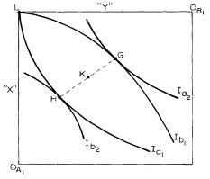
Figure 9

map shows indifference curves convex to, and transitive from, the intercept OB₁ . We assume an initial stock of rewards X and Y with entity A (the enterprise) controlling all of X and with entity B (the African government) controlling all of Y. Point L represents the initial distribution of X and Y; for example, the enterprise controls the revenue, and the government the basic resources.

The entities each might gain from an exchange of these rewards; each may prefer some distribution other than that indicated by point L, Which is acceptable to both individuals as an initial distribution. Exchange of X by A to B for Y could take place so that indifference curve

is followed downward to the right. If the exchange is conducted at point G, then B is made no worse off, but A will reach a more preferred position. At point G, indifference curve is tangential to indifference curve . A further exchange would result in a less preferred position for at least one party. Similarly, entity B could exchange at Y to entity A for X in a way so that indifference curve is followed downward to the right to point H. Such an exchange would leave A no worse off, but it would place B in a more preferred position. At point H, indifference curve is tangential to indifference curve and further exchange would result in a less preferred position for at least one entity.

There is a bargaining range between points G and H in Figure 9, and each point along this bargaining range (contact

---

curve) would move both partners to positions more preferable than at point L. This range of equilibrium distributions is traced out in a straight line from H to G. These points are on a contract curve formed by the points of tangency of A's indifference curves with B's. By equilibrium we mean an exchange at some point, such as K, which, when reached, will be maintained until there is a change in the value of the factors determining the bargaining terms. Two critical determining factors are impatience and reciprocal demand intensity. If A is "better situated" with respect to these factors, equilibrium will approach point G. The necessary conditions for the achieving of an equilibrium bargain is, first, that their indifference curves must be tangential and, second, that they are tangential where their slopes equal the slope of the terms-of-bargaining line. The terms-of-bargaining line represents the ratio at which one reward is exchanged for the other.

We shall next focus on the determination of the terms of bargaining by concentrating on time and the impatience and the reciprocal demand intensities of trading partners. We use the concept of the offer curve to assist us here. It is also a concept appropriated from economic theory. An offer curve shows the various ratios at which an entity is willing to exchange some quantity of a reward that the entity controls for a reward that the trader wants but does not control. We have noted that the determinants of these ratios (and consequently the offer curve) are impatience within the bargaining period and the reciprocal demand intensity for rewards in exchange. We begin with these assumptions: First, as the bargaining period draws to a close, each partner will offer its counterpart progressively more favorable bargaining terms to assure that some beneficial bargaining will be contracted; for example, the entity becomes more impatient. Second, the trading partners vary in their intensity of demand for "more preferred positions." Moreover, several other assumptions are required: (1) two bargaining entities exist; (2) two bargaining rewards, X and Y, exist and they are divisible; (3) bargaining is conducted to determine a mutually acceptable ratio at which X and Y are exchanged and divisibility of rewards is acceptable; (4) entity A controls all of reward X, and B all of Y; (5) costs of obtaining X and Y are identical for entities A

---

and B; (6) a given pattern of impatience and demand intensity for each entity is fixed, and each is unaware of the degree of the other's impatience and demand intensity; and (7) bargaining skills and experience of A and B remain fixed. In effect, we are analyzing only the impact of time and impatience and reciprocal demand intensity on the bargaining outcome. We could relax these assumptions in order to more closely depict actual bargaining cases. However, the implications regarding impatience and reciprocal demand intensity would be exactly as depicted under our strict assumptions.

In Figure 10, the vertical axis measures units of X and the horizontal axis measures units of Y from the zero intercept to some positive quantities. Offer curve

portrays the ratios at which entity A is willing to offer good X to entity B in exchange for good Y. The shape of the offer curve of A at each subperiod in the bargaining time-span indicates the ratios at which A is prepared to sacrifice some X to obtain some Y. The offer curve shows that entity A is willing to exchange a unit of X for 3 units of Y early in the bargaining period, but gradually becomes willing to offer relatively more units of X per unit of Y, or conversely, to accept relatively less of Y per unit of X. This is done to ensure that some bargain improving A's position will be contracted. At point K, bargainer A is willing to offer its item at an exchange ratio of 1X: 1Y at some time during

Figure 10

---

the bargaining period. Curve

portrays the ratios at which entity B is willing to exchange various quantities of Y to A for X at various subperiods throughout the bargaining span.

Entity B is assumed to behave similarly to A. Early in the bargaining period, B is willing to exchange Y at a ratio of three X for one Y. However, as time passes, individual B becomes progressively more willing and, at the time that the bargain is struck, this bargainer is also prepared to exchange at the ratio of 1Y:1X. At the end of each subperiod, the institutional structure within which the bargaining occurs permits, we assume, each entity to make explicit the ratio at which it is willing to exchange. In this case, an equilibrium exchange ratio of 1X:1Y is acceptable to each trading partner at the same time. This is shown at point K in Figure 10, and we note this as terms-of-trade line T₁ .

The terms of trade (established through offer curve analysis) relates to the determination of some equilibrium point along the contract curve (established through indifference analysis). In Figure 11, note that

and are tangential at point K. At this point each indifference curve is also tangential to terms-of-trade line T₁ which is determined at point K in Figure 10. At point K in Figure 11, each is better off than at point L. Each has been able to move transitively to a more preferred position, or to a higher indifference curve lying farther to the right on each indifference map. In moving from L

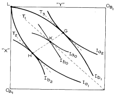
Figure 11

---

to K, each bargaining partner exchanges a portion of its initial reward distribution at a ratio of one unit of X for one unit of Y.

This particular exchange has put each entity in a preferred position. But it is not necessary that the offer curves of each have to be tangential at point K. They might choose to exchange at some other ratio, and if so, the resulting equilibrium point will not be K. For example, we now assume that entity A's offer curve is modified either because of its increasing impatience for some bargain to be struck or because it has increased the intensity of its demand for the reward wanted but not controlled. A's new offer curve is

and it is obtained from new data indicating that A is willing to give more units of X for every unit of Y. In this new case, A is willing to exchange at a ratio of 1.5X for 1Y. This is a ratio that entity B also finds acceptable. Thus a bargain is struck and it is one more favorable to B (or less favorable to A) than before A either became more impatient or demanded what B controlled more intensely. In both Figures 11 and 12, the equilibrium bargaining point is at H. It is the new terms of trade or exchange T₂ at which bargaining takes place and bargainer B obviously receives better terms of trade than before. Our African government, entity B, is in a more preferred position, but the opposite could well be the case if the government's bargainers became impatient or began to demand more intensely what bargaining party A, the MNC,

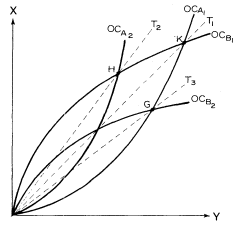
Figure 12

---

had to offer. In this situation, terms of bargaining would degenerate for the government, and as shown in Figures 11 and 12, the new terms of exchange would be T₃ and the equilibrium bargaining point G.

We are not unmindful of the difficulties associated with gaining more effective and preferential terms with MNCs.^[45] But it seems to us that the necessity of doing so is of overwhelming importance to African decision-makers. This point is clear from the recent agendas of the meeting of the Group of 77 in Manila and the more recent UNCTAD IV meetings in Nairobi.

[45] The bargaining process is much more complex than our simplified version. In the case of multinational copper companies in Chile, the bargaining outcome was a struggle of diverse groups interacting over a period of time. It was not confined to an omnipotent multinational giant and another bargainer called a host country. See Theodore H. Moran, Multinational Corporations and the Politics of Dependence: Copper in Chile (Princeton, N.J.: Princeton University Press, 1975). For an excellent analysis of an African situation, see Richard L. Sklar, Corporate Power in an African State: The Political Impact of Multinational Mining Companies in Zambia (Berkeley and Los Angeles: University of California Press, 1975).

---