PART THREE—
CRUSTAL TECTONICS AND THE DISTRIBUTION OF EARTHQUAKE FOCI
Nine—
Seismicity Map of North America
E. R. Engdahl and W. A. Rinehart
Introduction
The Decade of North American Geology (DNAG) is a special project commemorating the 1988 centenary of the Geological Society of America (GSA). Publications resulting from the project will include the twenty-eight-volume Geology of North America, a six-volume Centennial Field Guide Set, four Centennial Special Volumes, twenty-three Continent-Ocean Transects, and seven Continent-Scale Maps of North America. The map set includes a Geological Map of North America, Gravity Anomaly Map, Magnetic Anomaly Map, Seismicity Map, Stress Map, Neotectonic Map, Thermal Aspects Map, and an accompanying volume, Neotectonics of North America. The maps will be wall size (four 42" × 55" sheets per map), in color, and made on a common base map at a scale of 1:5,000,000.
A GSA-sponsored workshop was held at the 1984 Seismological Society of America meeting in Anchorage, Alaska, to discuss construction of the seismicity map. The consensus goal of the seismicity map is to provide a useful resource on North American seismicity for seismologists, for Earth scientists at the graduate level, and for industry. The objective is to portray accurately North American seismotectonic features using the entire earthquake history from the early 1500s (pre-instrumental) through the modern period. Thus, construction of the map data base requires the rationalization of hundreds of thousands of earthquake hypocenters from global, national, regional, and local catalogs. Since modern data are more useful than historic data for resolving seismotectonic features, a scheme of data selection and representation must be devised that reveals details of the seismotectonic fabric of North America yet preserves a perspective of historical earthquake occurrence. The problem is further complicated by the highly variable monitoring capa-
bility of seismic networks and by the different types and rates of occurrence of earthquake activity throughout North America.
A scheme was developed at the workshop using regional magnitude-completeness thresholds that vary with time for data selection, and a system of symbols and colors to portray seismicity data on the map. Local seismotectonic features of the map can be addressed on a regional basis in contributions to the accompanying volume, which includes small-scale maps and cross sections.
The goal of this paper is to present further details of the rationale used to construct the seismicity map in general and to assess several interesting elements of earthquake monitoring in the western United States.
Earthquake Data Bases
Catalog information on the occurrence of earthquakes usually includes parameters such as the origin time, location, focal depth, and magnitude or intensity of individual events. In the case of historic pre-instrumental earthquakes, these parameters must be determined entirely from intensity data and, hence, are less accurate than modern earthquake data. Presently, institutions around the world and in North America have varying degrees of responsibility for the collection and processing of earthquake data and for the catalog reporting of earthquake parameters on global, national, regional, and local scales.
On the global scale, the U.S. Geological Survey (USGS) and predecessor organizations (for example, the former U.S. Coast and Geodetic Survey) have been reporting the parameters of earthquakes worldwide within a few months of their occurrence through the Preliminary Determination of Epicenters (PDE) and earlier programs since 1928. The PDE program now routinely reports parameters for earthquakes as small as magnitude 4.5 worldwide and 3.5 within the conterminous United States. Two years after publication of the PDE reports, the International Seismological Centre (ISC)—prior to 1964, its predecessor the International Seismological Summary (ISS)—revises the PDE parameters and determines new events using a significantly larger data base. Global earthquake parameters have also been available from other sources such as the Bureau Central International de Séismologie (BCIS) and from special catalogs of larger earthquakes that often provide useful new information on the magnitudes of earlier events.
Prior to 1964, the global catalog of earthquake parameters is less complete, hypocenters are subject to greater uncertainty, and magnitude information is available for only the larger events. In 1964, with the advent of advanced computer processing of earthquake data and the installation of the Worldwide Standardized Seismograph Network (WWSSN), the reporting
of earthquake parameters was sharply advanced. The data base for areas in North America not monitored by regional networks relies heavily on global earthquake parameters reported since 1964.
On the national level, the USGS has compiled data on earthquake occurrence through the publications Earthquake History of the United States and the annual United States Earthquakes, and through special compilations used to construct state seismicity maps and for hazard analysis. The Geological Survey of Canada has a similar and continuing effort.
On regional and local scales, the data bases are somewhat more complicated. With regional network coverage in California, the University of California at Berkeley has cataloged the seismicity of northern and central California since 1910, and the California Institute of Technology has cataloged the seismicity of southern and central California since 1932. It was not until the 1960s in Canada and the 1970s in the United States that other regional networks in other parts of North America started to routinely compute the parameters of smaller earthquakes. Many of the regional institutions started upgrading their historical catalogs in the 1960s and 1970s, and some groups such as the California Division of Mines and Geology, the Electric Power Research Institute, and private consulting firms have attempted to combine the data from several networks into a single catalog. These efforts have all had to overcome, with varying degrees of success, the kinds of problems addressed in the next section. To our knowledge, the data base assembled for the North American Seismicity Map is the first attempt to combine comprehensively the earthquake data from all sources in North America into a single catalog.
Data Base Construction
One of the most formidable problems in assembling the North American data base is the association of entries in different catalogs for the same earthquake. For example, we often find that the parameters of larger earthquakes based on globally distributed stations are significantly biased relative to parameters determined by regional data alone. It is also common to find an overlap in regional network coverage so that parameters for the same earthquake are independently estimated by different networks. In many instances, the earthquake locations have different biases or are less accurately determined by one of the networks. To further complicate the problem, the differences are not systematic, but may vary between regions and in time.
Resolution of this problem required the development of a catalog hierarchy and subjective estimates of probable errors in origin time, location, and magnitude on a region-by-region basis. In the most general sense, preferred parameters for individual earthquakes are ranked in the order of local,
regional, national, and global estimates. Hierarchies in regions of overlap between networks are determined only after considerable discussion with regional experts.
In some cases, it is obvious that the same earthquake has been differently characterized in different catalogs. An origin-time error commonly found in data prior to 1964 is simply the difference between local and Greenwich mean time. There are also many one-hour errors due to changes between time zones, daylight savings time, and war time during World War II. One-minute errors in origin time are also common. Simple errors in origin time such as these are easy to identify, but other differences between catalogs require more careful individual attention. For example, locations for historical earthquakes are often quoted to only the nearest degree in some catalogs and to 0.25°, 0.5°, or 0.1° in others, resulting in large differences between locations. Even in modern catalogs, differences in regional location estimates for the same earthquake are sometimes found that are as large as 100 km because of regional network biases or poor determinations. Finally, very large magnitude differences, well beyond those that might be expected in the estimation of magnitudes by different methods, are often found between catalogs for earthquakes that appear to be the same.
The resolution of these difficulties had to be found by experimentation with origin time, location, and magnitude association windows that varied from one catalog to another and with region and time. For small windows, the association of earthquakes between catalogs for some previously determined hierarchy could be accomplished automatically. However, larger association windows were invariably needed to process historical data or to search for gross errors in modern data. In the latter case, the DNAG data base required the tedious examination of long lists of possible associations of earthquakes between catalogs on the basis of origin time, location, and magnitude. In this process, there are always some duplicate entries that cannot be resolved without the assistance of data contributors. This assistance was provided with varying degrees of thoroughness.
A number of different magnitude estimates are often reported for the same earthquake even in the same catalog. These magnitudes may be determined by using different methods and/or from different wave types not always easily related to one another. Frequently used magnitude scales include those based on estimates of the seismic moment (Mw ), on the maximum amplitudes of teleseismic body waves (mb ) and surface waves (Ms ), on the maximum amplitudes of local recordings (ML ), and on signal duration (MD ). As the earthquake size increases, many of these scales saturate, that is, reach a maximum value. For earlier, pre-instrumental earthquakes, only maximum intensities are known, which must be converted to magnitudes. Where necessary, we have converted maximum reported intensities to a magnitude (MI ) using MI = 1 + 2I0 /3 for the western United States and Canada and
M1 = 0.5(I0 + 3.5) east of the Rockies. To facilitate the assessment of reported magnitudes, we carry Ms , mb , and up to five reported magnitudes for each event in the database. For data selection and plotting, we use the largest reported magnitude of each event unless some other hierarchy has been suggested by a regional contributor. Any errors introduced by this approach are not serious as we plot only in magnitude-interval classes of one unit and, although the larger events are reviewed very carefully, we are not attempting to produce definitive magnitude estimates for each event.
Data Selection
It was recognized at the outset that plotting the entire historical record without accounting for changes in monitoring capability with time, or for the greater accuracy of modern data, would severely limit the usefulness of the seismicity map. For example, the expansion of regional networks and significant advances in processing of seismic data in the 1970s significantly lowered the magnitude threshold for seismicity data over large regions of the United States. On the other hand, we would like to know the locations, even though approximate, of larger-magnitude historic events relative to source zones that are well defined by low-magnitude modern seismicity data.
A solution to the problem was suggested by a seismic zonation of Canada for the purpose of seismic-risk estimation (Basham et al., 1985). The method requires the identification of spatially distinct earthquake source zones and the derivation of a magnitude-recurrence relation for each zone. A list of earthquakes can be selected for each zone on the basis of a magnitude-completeness test, that is, historical time periods over which earthquakes at different magnitude levels appear to be completely reported. We extend this concept to the case of regional network coverage as shown in figure 1, which displays generalized magnitude-completeness thresholds with time. This differs from the Basham et al. approach in that we are concerned with completeness of seismicity within regions now defined by regional network coverage and/or extensive cataloging of seismicity data, rather than within earthquake source zones that are spatially distinct. For a given time and region, only earthquakes with magnitudes large enough to be completely reported are selected for the DNAG seismicity map.
The benefits of such a scheme are numerous. It provides a natural selection of seismicity data that emphasizes larger earthquakes in the earlier historical period and smaller earthquakes in the more recent modern period. By a proper choice of symbol definition and scaling, as shown along the left margin of figure 1, we can see the relative levels of activity by scanning only the large symbols on the derived seismicity map, yet also see the fine detail provided by modern data. We further enhance the representation by using a darker shade for modern earthquake data. This enables viewers to easily
Figure 1
Generalized magnitude-completeness thresholds as a function of time.
Actual magnitudes of completely reported earthquakes for a given time
interval vary regionally (see figure 3). Symbol shading, definition, and
scaling help to preserve the seismotectonic perspective of the map.
draw their own conclusions about the relationship of larger historical earthquakes to sources of modern earthquakes. The scheme dramatically reduces the effect of changes in the seismicity base with time, but preserves the seismotectonic character of the map.
Regional Network Coverage
Figure 2 displays approximate regional network boundaries or source regions in the western United States over which variations in magnitude-completeness thresholds with time have been estimated. Especially active source zones, such as Mammoth (MAM) and Yellowstone (YSTON), have been isolated because of the considerable overlap in network coverage, and this often appears to artificially partition the regional network coverage (as, for example, the coverage of YSTON by the MBMG network). However, in every case, more than one catalog has contributed to the data base for a particular source region. For regions not covered by regional networks, we
Figure 2
Definition of approximate regional network boundaries or source regions in
western North America over which magnitude-completeness thresholds have
been estimated. Abbreviations (for example, SGB: Southern Great Basin, MEN:
Mendocino, and MAM: Mammoth Lake) are arbitrary since, in every case, more
than one catalog contributed to the data base for a particular source region.
Figure 3
Magnitude-completeness thresholds versus time for selected western North
America networks or source zones. The period prior to the 1920s is incomplete
but includes all known earthquakes of maximum intensity seven or greater. The
separation of modern and historical data (arrows) usually occurs in the 1970s.
used magnitude thresholds developed by Dewey et al. (1987) for a framework study. They use a uniform magnitude threshold of 3.5 for the conterminous United States since 1975, when regional network coverage expanded and the USGS initated a project to recover source parameters of all U.S. earthquakes to that level.
Variations in magnitude-threshold estimates with time are shown for selected western United States networks in figure 3. Some networks have produced rigorous analyses of their monitoring capability, but in most cases completeness thresholds with time are based entirely on the subjective judgment of regional experts. The period prior to the 1920s is known to be incomplete for all regional compilations. However, because of the importance of some of the moderate-size earlier earthquakes, we have, unless otherwise specified, set the magnitude threshold for the earlier period low enough to include all known earthquakes of maximum intensity 7 (MI = 5.75) or greater in the western United States. To provide some measure of homogeneity on the map, we plot only earthquakes of magnitude 2.5 or above in regions such as southern Nevada and central California, where the magnitude-
completeness threshold might be as low as magnitude 2 in the modern period. The separation of modern and historical data usually occurs in the 1970s when magnitude-completeness thresholds were significantly lowered by the installation of regional networks.
Seismicity Map
Figure 4 is a seismicity map for the western United States produced by the scheme previously described. Since detailed interpretations will be published elsewhere (for example, Dewey et al., 1987, and the volume accompanying the DNAG map set), we will attempt to describe only the highlights revealed by this map.
Regional patterns of seismicity in the part of the western United States shown in figure 4 can be interpreted within the context of plate-tectonic models. With modern high-resolution seismicity data, it is now possible to relate these patterns to local and global tectonic processes and to associate earthquakes with geologically mapped faults or other geologic structures. For example, in figure 4 northwest trending lineations of epicenters associated with right-lateral faults in California are superimposed on a background of more widely scattered epicenters and clusters of epicenters. Moreover, the rate of seismicity differs between zones that are approximately delineated by major structural provinces.
It is also quite evident that without the historical data the perspective of earthquake occurrence in time is lost or distorted. For example, sections of the San Andreas ruptured by major earthquakes in 1857 and 1906 are now relatively quiet, even at the lower magnitudes. On the other hand, some source zones, such as the region off Cape Mendocino and the Mammoth area, have clearly been highly seismic over the entire historical record. Larger historical earthquakes fold into the seismic patterns quite well, and inferences on their relationship to modern earthquake patterns (or lack thereof) are made possible.
Overall, the map achieves the desired objective. It displays fine details of the seismicity revealed by modern high-resolution data yet preserves information about historical earthquake occurrence. The result is an accurate portrayal of the seismotectonic fabric of the region over the period for which we have a recorded history.
Discussion
Construction of the DNAG Seismicity Map of North America has revealed important facets about earthquake monitoring in the western United States.
For the most part, the western United States, including the Rocky Mountain region, is reasonably well monitored by present-day networks. Areas monitored to only about the magnitude 3.5 level include Oregon, large parts
Figure 4
Seismicity map of part of western North America produced by the scheme described
in the text. Relative symbol scaling is identical to that used for the DNAG Seismicity
Map of North America. Historical data are more lightly shaded than modern data.
of Idaho, and Arizona. These are regions of low seismicity in which funding agencies have not been inclined to support the installation of permanent networks (although some short-term studies have been made). The offshore regions, especially west of about 126° near Cape Mendocino, obviously pose a special problem and are complete only to relatively high teleseismic magnitude thresholds.
There is considerable overlap in network coverage over large areas of the western United States. Networks in California and Nevada apparently share phase data, and in some cases the actual data stream, but individual catalogs often extend beyond their network boundaries, and there is considerable uncertainty in the choice of preferred hypocenters. To some extent, there is a duplication of effort, but this is probably desirable to insure continuity in the overall catalog. Somewhat better coordination exists between the United States and Canada in the Pacific Northwest, and Mexico in the Baja California region.
The users of regional network data in the western United States could certainly benefit through improved usage of magnitudes and better regional recurrence estimates. The types of magnitudes commonly used vary, and relationships between them are not well known. Some standardization seems essential. In most cases, network magnitude thresholds as a function of time are only subjective estimates. It is possible and necessary to perform a more careful analysis over well-defined regions.
Finally, a coordinated effort is needed to correct and update the DNAG data base for the western United States. This will require better definition of variations in network coverage with time, determination of more accurate regional magnitude-completeness thresholds, and some attempt to rationalize the differences between reported magnitudes.
Acknowledgments
We thank G. Reagor for invaluable assistance in the preparation of catalog data for entry in the U.S. Geological Survey computer-based Earthquake Information System. J. W. Dewey, J. N. Taggart, and C. Stover are thanked for helpful reviews and suggestions.
References
Basham, P. W., D. H. Wiechert, F. M. Anglin, and M. J. Berry (1985). New probabilistic strong seismic ground motion maps of Canada, Bull. Seism. Soc. Am., 75: 563–595.
Dewey, J. W., D. P. Hill, W. L. Ellsworth, and E. R. Engdahl (1988). Earthquakes, faults, and the seismotectonic framework of the contiguous United States. In L. C. Pakiser, and W. D. Mooney, eds., Geophysical Framework of the Continental United States, GSA Memoir.
Ten—
Seismicity of the Australian Plate and its Pacific Plate Margin
David Denham
Introduction
The patterns revealed in plots of earthquake hypocenters are crucial for interpreting tectonic processes within the Earth. At active plate boundaries, where a satisfactory model has been developed, hypocentral locations provide inportant information on tectonic details. Even in complicated areas, studies of the spatial distribution of earthquakes can provide considerable information on the geometries of the plate margins and the subduction zones. In the New Guinea region, for example, where the Australian and Pacific plates interact strongly, there is not one simple plate boundary but a cluster of small plates, each boundary accommodating a component of the total interaction. Furthermore, there is not one single subduction zone but several. For the Australian continent, however, which is an intraplate environment, there is no comparable tectonic model to successfully interpret the seismicity patterns. We know very little about the causes of this seismicity, except that the earthquakes are all shallow and caused by compressive forces, and that large earthquakes can and do occur in the Australian region. The task of developing a successful model to describe intraplate seismicity patterns is one of the most important seismological problems to be tackled in the next decade.
Background
It is fitting, in this centennial anniversary symposium, that the first session is devoted to the mapping of earthquakes. For if one examines the advances associated with matters seismological, it is clear that these have, in many instances, depended on the available capability to locate and map earth-
quake hypocenters. Readers need hardly be reminded of the role played by seismology and seismologists in the development of plate tectonics, and how the delineation of plate boundaries was achieved by interpreting the spatial patterns of hypocenters. It was not enough to simply plot the hypocenters; it was necessary to interpret the patterns in terms of a meaningful model. Thus we have another example of the old adage that you see only what you know, and I suppose if any theme characterizes this paper, this is it. If you can fit the observations to a model, then all is well; if you can't, you have problems.
What I intend doing is to look at two regions associated with the Australian plate and demonstrate how, over the past eighty years or so, our improved capabilities to map earthquakes have led to an enhanced understanding of the tectonic processes in one region, where we have a model, and have led to little progress in the other region because we don't have a model. The two regions are the northern margin of the plate in the vicinity of New Guinea, and that part of the Australian plate occupied by the Australian continent (fig. 1).
Papua New Guinea
The first publication on the seismicity of Papua New Guinea was probably Sieberg (1910), which was based largely on reports of earthquakes from the church missions established there close to the turn of the century. He listed twenty-four earthquakes that occurred in the period 1900–1906 (fig. 2). He even attempted to interpret the seismicity in terms of the tectonics of the region. However, apart from recognizing that "New Guinea and the Bismarck Archipelago form part of the innermost arc of young folded mountains which approach the rigid Australian platform," his general conclusion was that "our knowledge is very deficient in this respect, because only sporadic observations are available."
By the time Gutenberg and Richter's Seismicity of the Earth was published in 1954 the data set had improved considerably, and most epicenters were computed using arrival times recorded at seismographic stations. They used a time window from 1904 to 1952 and came close to relating earthquakes to a plate-tectonic type of activity. For example, they recognized (pp. 97–101) that "Most of the earth's surface is partitioned among a number of comparatively stable blocks, separated by active belts" and "the foci of deep shocks seem to be restricted to the vicinity of a nearly plane surface, which is probably related to a thrust surface between two different structures, usually dipping towards the continent." However, they mistakenly suggested that the midocean ridges "can hardly be young structures" even though they recognized that in the case of the mid-Atlantic ridge "Its parallelism with the continental coasts is so close that it practically demonstrates a mechanical connection with them." It is interesting to note that in the Papua New
Figure 1
The Australian plate and its boundaries. Area 1 defines the New
Guinea region and Area 2 the Australian continent, the two
regions discussed in the text. Arrows indicate the directions
of plate motion relative to the Antarctic plate.
Figure 2
New Guinea epicenters for 1900–1906 (Sieberg, 1910).
Guinea region the main features of the shallow, intermediate (70–300 km), and deep (> 300 km) earthquakes had by then been determined, which is quite remarkable when one considers the extent of the global network in the pre-1950s, and also the absence of any regional stations at that time.
In Japan, meanwhile, Wadati (1934), using data from regional stations, had been able to define quite precisely the zone of earthquakes dipping beneath Honshu, and had also suggested that "This tendency seems to be observable in many volcanic regions in the world. Of course, we cannot say decisively but if the theory of continental drift suggested by A. Wegener be true, we may perhaps be able to see its traces of the continental displacement in the neighbourhood of Japan"—not bad for 1934.
In New Guinea, the next study after Gutenberg and Richter was made by Brooks (1965) who applied data from 1906 to 1962 to earthquake risk assessments. His results do not represent a significant improvement over Gutenberg and Richter's earlier work. However, Denham (1969) used data from the period 1958–1966 in an attempt to interpret the hypocentral patterns in terms of the fledgling plate-tectonic theories being developed at the time. Figure 3 shows his results. There is a significant improvement in the definition of the lineations, and it is clear that the northern boundary of the Australian plate is not a simple boundary. The reasons for the improvements in the data set were mainly due to the establishment of the Worldwide Standardized Seismographic Network (WWSSN) in the late 1950s and early 1960s and the computing facilities of the U.S. Coast and Geodetic Survey (USCGS). Some indication of the improvements may be gauged from the fact that only 256 events from the region were listed by Brooks (1965) for the period 1906–1962, whereas in 1966 alone 309 earthquakes were located in the same region by the USCGS.
Denham (1969) was able to identify the zones of deep and intermediate-depth earthquakes associated with the volcanic arcs and also the Bismarck Sea Seismic Zone (BSSZ). This is defined by the line of epicenters extending from 143° E to 152º E at 3° S. However, the northern boundary of the Aus-
Figure 3
New Guinea epicenters for 1958–1966 earthquakes with M ³ 5 (Denham, 1969). BSSZ indicates the Bismarck Sea Seismic Zone, and SS indicates the Solomon Sea.
tralian plate was probably misidentified as being along the northern coast of the island of New Guinea and the northern margin of the Solomon Sea (SS).
As shown in figure 4, compiled from more recent data, this interpretation is probably not correct. The northern margin of the Australian plate is situated farther to the south. In figure 4 all epicenters located by twenty or more stations since 1970 have been plotted. The improved regional seismographic coverage since that date has revealed a zone of seismicity in the central part of the main island of New Guinea (A-Á in fig. 4a) and another zone near the East Papuan peninsula (see Ripper and McCue, 1983). These diagrams indicate the details that can be revealed with a good-quality data base. Each lineation can be interpreted in terms of plate tectonics and the interpreta-
tions checked by analyzing fault-plane solutions and observations of recent crustal movements.
At depths between 70 and 300 km the hypocentral lineations are equally well determined and can be interpreted in terms of subducting lithosphere (fig. 4c). Similarly, for earthquakes deeper than 300 km (fig. 4d) the slabs (or what is left of them) are also clearly identified.
Therefore, in a plate margin situation, even though the tectonics are complicated it is possible to use the spatial distributions of earthquake hypocenters to unravel the current dynamics of the region. Such inferences are not possible in an intraplate environment where no suitable model for earthquake occurrences has as yet been developed.
Figure 4
New Guinea epicenters for 1970–1984 where twenty or more
stations have been used to locate the hypocenters.
(a) Shallow (0–50 km) earthquakes with coastlines. A–Á
indicates the northern margin of the Australian plate
in the center of New Guinea.
(b) Shallow earthquakes without coastlines.
(c) Intermediate Depth (70–300 km) earthquakes
without coastlines.
(d) Deep (> 300 km) earthquakes without coastlines.
Notice how the shallow earthquakes define the plate and
subplate boundaries, and the intermediate and deep
earthquakes define the subducted slabs.
Australian Continent
Earthquakes have been reported from the Australian continent since the First Fleet landed in 1788, but it was not until 1952 that a study of Australian seismicity was published (Burke-Gaffney, 1952). This was followed by Doyle et al. (1968), whose comprehensive study listed 165 earthquakes in the period 1897 through 1966. This data set is not large enough to determine any meaningful patterns.
If we examine a more recent data base including earthquakes through 1984, the situation is essentially unchanged (fig. 5). The epicentral patterns, or lack of them, are difficult to interpret in terms of a tectonic model. It is clear that most of the earthquakes occur within the continent, but the patterns of epicenters do not appear to correlate with any significant geological feature. Figure 5a shows the distribution of earthquakes and the main geological features, and figure 5b shows the earthquakes without visual distractors. Although there are several hundred epicenters, it is difficult to develop any continent-wide model that describes the occurrences. However, we can make the following statements.
1. The earthquakes in the Australian region appear, for the most part, to be restricted to areas of continental crust (Lambeck et al., 1984).
2. The patterns appear to define regions of comparatively high seismicity, which surround regions of lower seismicity.
3. All onshore earthquakes occur in the upper 20 km, and most are in the upper 10 km (Lambeck et al., 1984).
4. Although in some small areas the earthquakes appear to be associated with known faults (Bock and Denham, 1983), in many instances—particularly for large earthquakes—there is no apparent correlation between the earthquakes and pre-existing faults.
5. All reliable focal mechanisms obtained to date (thirty-eight) are consistent with the presence of compressive stress in the crust—confirmed by in-situ stress measurements and surface-faulting observations (Denham, 1986; Lambeck et al., 1984).
Figure 5
Australian epicenters of magnitude 4 or
greater earthquakes, 1873–1985,
(a) showing the main geological features and
(b) without visual distractors. Notice
how the epicenters appear to group around
areas that have experienced no earthquakes.
Apart from these statements, which describe particular aspects of the seismicity in the Australian region, I would conclude that at present there is no reliable model to describe the overall space-time earthquake patterns.
Discussion and Conclusions
At the northern boundary of the Australian plate, in the Papua New Guinea region, even though the tectonics are complicated, detailed and accurate mapping of earthquake hypocenters can provide important information on the plate boundaries and subduction zones. This is because the patterns can be interpreted in terms of a known plate-tectonic model. However, for the Australian continent, which is an intraplate environment, there is no comparable model that can be used successfully to interpret the seismicity patterns. Thus, the development of a successful model to describe intraplate seismicity patterns is one of the most important seismological tasks to be tackled in the next decade, because large earthquakes can and do occur in intraplate regions.
Acknowledgment
I thank the Director, Bureau of Mineral Resources, Geology and Geophysics, for permission to publish.
References
Bock, G., and D. Denham (1983). Recent earthquake activity in the Snowy Mountains region and its relationship to major faults. J. Geol. Soc. Australia, 30: 423–429.
Brooks, J. A. (1965). Earthquake activity and seismic risk in Papua and New Guinea. Australian Bureau of Mineral Resources, Geology & Geophysics, Report No. 74.
Burke-Gaffney, T. N. (1952). Seismicity of Australia. Journal and Proceedings of the Royal Society of New South Wales, 85: 47–52.
Denham, D. (1969). Distribution of earthquakes in the New Guinea-Solomon Islands region. J. Geophys. Res., 74: 4290–4299.
——— (1986). Stress patterns in the Australian continent—Evidence from earthquakes, borehole deformations, and in-situ stress measurements, (abstract). In Earthquake Notes 57: 5.
Doyle, H. A., I. B. Everingham, and D. J. Sutton (1968). Seismicity of the Australian continent. J. Geol. Soc. Australia, 15: 295–312.
Gutenberg, B., and C. F. Richter (1954). Seismicity of the Earth and Associated Phenomena. Princeton University Press, Princeton, N.J., 310 pp.
Lambeck, K., H. W. S. McQueen, R. A. Stephenson, and D. Denham (1984). The state of stress within the Australian continent. Annales Geophysicae, 2: 723–742.
Ripper, I. D., and K. F. McCue (1983). The seismic zone of the Papuan fold belt. BMRJ. Australian Geol. Geophys., 8: 147–156.
Sieberg, A. (1910) Die Erdbebentatigkeit in Deutsh-Neuguinea (Kaiser-Wilhelmstand und Bismarck-archipel). Petermanns Geographische Mitt., II, Heft 2/3.
Wadati, K. (1934). On the activity of deep-focus earthquakes in the Japan Islands and neighborhoods. Geophys. Mag., 8: 305–325, Tokyo.
Eleven—
State of Stress in Seismic Gaps along the San Jacinto Fault
Hiroo Kanamori and Harold Magistrale
Introduction
Data from the Southern California Seismic Network have been extensively used to map spatial and temporal variations of seismicity (for example, Hileman et al., 1973; Green, 1983; Webb and Kanamori, 1985; Doser and Kanamori 1986; Nicholson et al., 1986). A recent study by Sanders et al. (1986) clarified some of the important features of historical seismicity along the San Jacinto fault of southern California, one of the most prominent being the Anza seismic gap. Thatcher et al. (1975) investigated the spatial distribution of large earthquakes along the fault and indicated that a 40-km-long section from Anza to Coyote Mountain is deficient in seismic slip and can be considered a seismic gap (G1 in fig. 1). Sanders and Kanamori (1984) investigated the seismicity along an 18-km-long section (also often called the Anza seismic gap) centered near the town of Anza, and concluded that this section of the fault is locked and has the potential for a magnitude 6.5 event (G2 in fig. 1).
In this paper, we review the most recent activity along the San Jacinto fault and assess the seismic potential of this fault zone in light of an empirical relation between fault length, seismic moment, and repeat time obtained from earthquakes along active fault zones around the world.
Recent Seismicity along the San Jacinto Fault
Figure 1, a map of recent seismicity along the San Jacinto fault, does not clearly show the seismic gap. Figure 2 is a cross section of the seismicity along the strike of the fault and includes all the events between points A and A' in the narrow box shown in figure 1. A similar figure has been presented
Figure 1
Seismicity along the San Jacinto fault, Southern California, for the period January 1,
1987, to June 30, 1987. The data are taken from the catalog of the Southern California
Seismic Network. All the events in the polygon are shown. The narrow box A–Á
indicates the area used for the cross-sectional plot shown in figure 2. Geographical
locations of the fault and the gaps are shown in the figure at the bottom.
by Sanders (1986) for an earlier time period. The most striking feature of these displays is the almost complete absence of seismic activity over an 80-km-long section (G3 in figs. 1 and 2) that includes the "Anza seismic gap." The only activity in this quiet zone is at a depth of about 13 km. Doser and Kanamori (1986) interpreted this activity to represent the bottom of the seismogenic zone along the San Jacinto fault.
We examined the seismicity in this zone for the period from July 1983 to December 1986 and found essentially the same seismicity pattern shown in figure 2.
The historical seismicity along this segment was reviewed by Thatcher et al. (1975), Sanders and Kanamori (1984), and Sanders et al. (1986).
Figure 2
Seismicity cross section along the San Jacinto fault (lower figure). All the
events in the box A–Á in figure 1 are shown. Three gaps, G1, G2, and G3,
are indicated. The upper figure shows the variation of heat flow along the
San Jacinto fault, taken from Lachenbruch et al. (1985).
Although the exact locations and sizes of the 1899, 1918, and 1923 events are uncertain, it is generally agreed that no large (ML > 6.5) earthquake has occured in the 80-km quiet section at least since 1918.
Another notable feature in figure 2 is the steady increase in the depth of the seismogenic zone, as defined by the deepest activity, from the south to the north. Doser and Kanamori (1986) interpreted this trend in terms of a depression of the geotherm evidenced by a decreasing heat flow. The heat flow along the San Jacinto fault taken from Lachenbruch et al. (1985) is shown in figure 2.
Interpretation
The seismicity pattern shown in figure 2 suggests that strain is building up in the locked fault zone at depths shallower than 13 km. The steady activity at the bottom of the seismogenic zone may be a manifestation of stress accumulation that will eventually cause failure of the overlying locked zone.
A similar seismicity pattern was observed before the 1979 Imperial Valley earthquake (M L > 6.5). Doser and Kanamori (1986) relocated earthquakes along the Imperial fault. Figure 3 shows the cross section of seismicity along the strike of the Imperial fault for a period of about two years before the October 15, 1979, earthquake. The solid curve in the figure outlines the slip
Figure 3
Cross section of seismicity along the strike of the Imperial fault for the period July
1977 to October 15, 1979. The hypocenters with A and B quality listed in the
Southern California Network catalog, relocated by Doser and Kanamori (1986),
are shown. The regions of the fault outlined by solid and dashed lines represent
strike-slip offsets of one meter from the rupture models of Hartzell and Heaton
(1983) and Archuleta (1984), respectively. E denotes the ends of the surface
faulting and B the intersection of the Brawley fault with the Imperial fault.
zone of the main shock where the strike-slip displacement exceeded one meter (Hartzell and Heaton, 1983). Because of the limited station distribution of the network, the events between DL and the hypocenter, located to the south of the United States–Mexico border, could not be relocated and are not shown in figure 3. This pattern also suggests stress accumulation beneath the locked portion of the Imperial fault.
Given this loading mechanism, we can assess the state of stress in the seismic gaps along San Jacinto fault in the following manner. If we assume that the strain is accumulating on a fault of length L and width W , the accumulated seismic moment M0 is given by

where µ is the rigidity, taken to be 3 × 10¹¹ dyne/cm2 , V is the slip rate, and T is the elapsed time since the last earthquake. If we take the entire 80-km quiet zone (G3) as a locked segment, then W = 13 km and L = 80 km.
Although the slip rate along the entire San Jacinto fault is not known accurately, Sharp (1981) indicates a minimum Quaternary long-term slip rate of about 8 to 12 mm/year for the segment in the vicinity of Anza. A slip rate of 1 cm/year seems to be a reasonable estimate.
Geodetic studies of King and Savage (1983) indicate an accumulation of
Figure 4
The relation between the fault length and seismic moment of shallow strike-
slip earthquakes in active plate boundaries. The dashed line indicates a
slope of 1/3 expected for the standard scaling relations. Closed and open
circles are the data taken from Kanamori and Allen (1986) and Scholz et al.
(1986), respectively. The horizontal lines indicate current strain
accumulation in the seismic gaps along the SanJacinto fault.
right-lateral strain in this area at a rate of 0.3 µ strain/year. No surface fault creep has been measured for at least the last ten years along the San Jacinto fault near Anza (Louie et al., 1985; see also Sanders and Kanamori, 1984).
These observations suggest a steady strain accumulation in this gap for at least seventy years since the last large earthquake in 1918. Substituting T = 70 years into equation (1), we obtain M0 = 2.2 × 1026 dyne-cm (corresponding to Mw = 6.8) as the minimum accumulated seismic moment along this segment. If the 1918 event did not break this segment, the cumulative moment could be even larger.
The next question is how close the presently accumulated strain is to the ultimate failure strain. We examine this problem on the basis of empirical data obtained from other earthquakes. Kanamori and Allen (1986) examined the relation between the fault length and seismic moment of shallow crustal earthquakes and found that, for a given fault length, earthquakes with longer repeat times have larger seismic moments than those with shorter repeat times. They interpreted this relation in terms of the difference in the strength of fault zones. Fault zones with longer repeat times are stronger than those with shorter repeat times. If we consider only the events with relatively short (less than 500 years) repeat times, a systematic relation can be obtained.
Figure 4 shows the relation between fault length L and seismic moment
M0 of shallow strike-slip earthquakes with repeat times less than 500 years in the world. The open and closed circles indicate the data taken from Scholz et al. (1986) and Kanamori and Allen (1986), respectively.
The seismic moments accumulated in the two segments (G2 and G3) of the San Jacinto fault are indicated in the figure. As the time elapses, the accumulated moment increases along the horizontal line drawn for the given fault length. If the strength of the San Jacinto fault zone is comparable to that of other fault zones, the fault should break when the head of the arrow (point P) reaches the moment value defined by the average trend of the data. Since the seismic moment is generally considered to be proportional to the seismic-wave energy released in earthquakes, we use the term "energy" below in place of "moment."
Figure 4 shows that the strain energy presently accumulated along the longer gap (G3) is at least comparable to the average of the ultimate strain energy that can be stored in an 80-km fault segment. In this sense, one can conclude that this gap is close to failure. We note, however, that the empirical data indicate a factor-of-two spread in strain energy, suggesting that strain accumulation can continue for another seventy years or so without breaking this gap.
Another possibility is that the strain is not uniform along the gap because of varying slip histories, so that only a part of the gap may break in a smaller earthquake. We can estimate the accumulated strain for this case using equation (1), but some ambiguity exists in the width W. The empirical relation shown in figure 4 suggests that W is not constant, but is approximately proportional to L (see Scholz, 1982; Kanamori and Allen, 1986). Equation (1) then suggests that the accumulated energy is proportional to L 2 . In figure 4 we show a straight line with a slope of 1/2 passing through point P. This line determines the level of strain accumulation for gaps with different lengths. For example, for the shorter Anza gap (G2) L = 18 km, and the accumulated moment is about M0 = 1 × 1025 dyne-cm (Mw= 5·9). If a gap with L = 40 km breaks, then M0 = 5 × 1025 dyne-cm (Mw = 6.4).
Conclusion
A comparison of the size of the gap and the elapsed time since the last large earthquake with fault length-moment relations of shallow strike-slip earthquakes suggests that the strain energy accumulated in the 80-km seismic gap along the San Jacinto fault is comparable to the ultimate strain energy that can be stored there. However, the ultimate strain per unit volume of the earth's crust depends on the strength of the fault zone. The empirical relation indicates approximately a factor-of-two variation in the strength for faults in active plate boundaries. This range translates into a factor-of-two variation in repeat time. It is therefore possible that strain accumulation could continue for another seventy years or so without causing an earthquake.
Other possible scenarios include: 1) The present slip rate along the San Jacinto fault is much smaller than 1 cm/year, and it takes much longer than seventy years to accumulate enough strain to break the gap. 2) The depth of the seismogenic zone is significantly greater in this segment than elsewhere along the San Jacinto fault, as evidenced by the decrease in heat flow, resulting in an increase in the overall strength of the fault zone and in the repeat time. 3) The 1899 and 1918 earthquakes did not completely break this gap, and the accumulated strain is larger than indicated in figure 4. In this case, the gap is closer to failure than indicated by figure 4. 4) The 40-km-long gap may fail in several smaller earthquakes.
Despite this uncertainty inherent in the empirical methods, the information obtained from detailed analyses of seismicity and earthquake rupture processes provides an important clue to the state of stress in a seismic gap with respect to its ultimate strength.
Earthquake prediction on the basis of empirical methods like the one presented above, and many others currently used, is obviously of limited accuracy. Nevertheless, it provides a physical framework for further experiments. In the case of the seismic gaps along the San Jacinto fault, high-resolution seismicity studies have delineated the geometry of the gaps and the currently seismogenic zone, which has enabled us to determine the physical condition of the fault (Sanders and Kanamori, 1984; Doser and Kanamori, 1986). Detailed analysis of the rupture parameters of earthquakes in similar tectonic environments provides a tool to measure the level of strain accumulation relative to the ultimate strain.
Obvious next steps involve more physical measurements. Since earthquakes are ultimately caused by strain accumulation, continuous monitoring of the strain field in the gap area is crucial. Also, since fault ruptures appear to initiate from the bottom of the seismogenic zone, studies of spatial and temporal variations of source characteristics of the events near the bottom of the seismogenic zone are important.
Acknowledgments
This research was partially supported by U.S. Geological Survey grant 1408-0001-G1354. Contribution number 4505, Division of Geological and Planetary Sciences, California Institute of Technology, Pasadena, California 91125.
References
Archuleta, R. J. (1984.). A faulting model for the 1979 Imperial Valley earthquake. J. Geophys. Res., 89: 4559–4585.
Doser, I. D., and H. Kanamori (1986). Depth of seismicity in the Imperial Valley
region (1977–1983) and its relationship to heat flow, crustal structure, and the October 15, 1979, earthquake. J. Geophys. Res., 91: 675–688.
Green, S. M. (1983). Seismotectonic study of the San Andreas, Mission Creek, and Banning fault system. Master's thesis, University of California, Los Angeles, 52 pp.
Hartzell, S. H., and T. H. Heaton (1983). Inversion of strong ground motion and teleseismic waveform data for the fault rupture history of the 1979 Imperial Valley, California, earthquake. Bull. Seism. Soc. Am., 73: 1553–1584.
Hileman, J. A., C. R. Allen, and J. M. Nordquist (1973). Seismicity of the South California Region, 1 January 1932 to 31 December 1972. Seismological Laboratory, California Institute of Technology.
Kanamori, H., and C. R. Allen (1986). Earthquake repeat time and average stress drop. In S. Das, J. Boatwright, and C. H. Scholz, eds., Maurice Ewing volume 6, Earthquake Source Mechanics. American Geophysical Union, Washington D.C., 227–235.
King, N. E., and J. C. Savage (1983). Strain rate profile across the Elsinore, San Jacinto, and San Andreas faults near Palm Springs, California. Geophys. Res. Lett., 10: 55–57.
Lachenbruch, A. H., J. H. Sass, and S. P. Galanis, Jr. (1985). Heat flow in southernmost California and the origin of the Salton Trough. J.Geophys. Res., 90: 6709–6736.
Louie, J. N., C. R. Allen, D. C. Johnson, P. C. Haase, and S. N. Cohn (1985). Fault slip in southern California. Bull. Seism. Soc. Am., 75: 811–833.
Nicholson, C., L. Seeber, P. Williams, and L. Sykes (1986). Seismicity and fault kinematics through the eastern Transverse Ranges, California: Block rotation, strike-slip faulting, and low-angle thrusts. J. Geophys. Res., 91: 4891–4908.
Sanders, C. O. (1986). Seismotectonics of the San Jacinto fault zone and the Anza seismic gap. Ph.D thesis, California Institute of Technology, Pasadena, 180 pp.
Sanders, C. O., H. Magistrale, and H. Kanamori (1986). Rupture patterns and preshocks of large earthquakes in the southern San Jacinto fault zone. Bull. Seism. Soc. Am., 76: 1187–1206.
Sanders, C. O., and H. Kanamori (1984). A seismotectonic analysis of the Anza seismic gap, San Jacinto fault zone, southern California. J. Geophys. Res., 89: 5873–5890.
Scholz, C. H. (1982). Scaling relations for strong ground motion in large earthquakes. Bull. Seism. Soc. Am., 72: 1903–1909.
Scholz, C. H., C. A. Aviles, and S. G. Wesnousky (1986). Scaling differences between large interplate and intraplate earthquakes. Bull. Seism. Soc. Am., 76: 65–70.
Sharp, R. V. (1981). Variable rates of late Quaternary strike-slip on the San Jacinto fault zone, southern California. J. Geophys. Res., 86: 1754–1762.
Thatcher, W., J. A. Hileman, and T. C. Hanks (1975). Seismic slip distribution along the San Jacinto fault zone, southern California and its implications. Geol. Soc. Am. Bull., 86: 1140– 1146.
Webb, T. H., and H. Kanamori (1985). Earthquake focal mechanisms in the eastern Transverse Ranges and San Emigdio Mountains, southern California, and evidence for a regional decollement. Bull. Seism. Soc. Am., 75: 737–757.
Twelve—
The Need for Local Arrays in Mapping the Lithosphere
A. Eisenberg, D. Comte, and M. Pardo
Introduction
There has been a significant effort in recent years to establish global arrays of broadband seismographs. Although the benefit of this kind of instrumentation has become quite obvious, it is also important to improve local arrays.
In this chapter, data from aftershocks of the Chile earthquake of March 3, 1985, and some additional 1981 earthquakes are used to analyze some important details of the tectonics of central Chile.
Locations for the aftershocks of the 1985 earthquake are derived using only phase arrival times from local seismograph stations, and these are compared with locations for the same earthquakes determined using data recorded principally at teleseismic distances. It is shown that the local array hypocenters outline the central Chile Benioff zone much more clearly than solutions that depend on worldwide data, even when such useful algorithms as Joint Hypocenter Determination are used.
Some 1981 Chile earthquakes, too small to be recorded except by an array of local seismographs, yield focal mechanisms that suggest several breaks or flexures in the descending lithosphere south of 33°S latitude.
These features are not apparent when only larger teleseismically recorded events are considered.
Earthquake Locations
The Chile earthquake of March 3, 1985, provided an opportunity to study the tectonics of central Chile using local seismographic network data. Prior to the earthquake, a permanent network of ten stations, operated and maintained by the University of Chile, had been installed to study the Pocuro
Figure 1
Permanent seismographic network of the University of Chile
and temporary portable stations from UNAM installed after the
March 3, 1985, central Chile earthquake.
fault that runs through the foothills of the Andes Cordillera. These stations are all east of the coastal region where the March earthquake occurred.
In order to better study the aftershock sequence of this event, the tenstation permanent array was supplemented by eight portable stations brought to the coast by scientists from the National Autonomous University of Mexico (UNAM). Both permanent and temporary station sites are shown in figure 1.
The 380 well-determined aftershock locations found from the data of this eighteen-station array are shown in figure 2. These epicenters were calculated using the flat layered crustal velocity model of Acevedo and Pardo (1985), with corrections in the form of P-wave and S-wave time delays at each array station, to compensate for the Earth's curvature. Only aftershocks with total recorded durations greater than 100 seconds and standard deviations in the final location of less than 0.5 seconds are plotted. S-wave arrival times were used in the locations of all 380 aftershocks.
A number of interesting features are shown by the 380 aftershocks of
Figure 2
Location of 380 aftershocks of the March 3, 1985,
earthquake using local-network data.
figure 2. First, earthquakes with depths less than 20 km are located mainly toward the deep marine trench that marks the margin between the Nazca and South American plates. Exceptions to this rule are a few shallow earthquakes occurring nearer the coast in the northernmost part of the aftershock zone.
Second, there is a concentration of inland earthquakes with focal depths greater than 30 km to the south of 33ºS. These events could indicate a bending or breaking of the downgoing slab.
Third, there are regions relatively devoid of aftershocks to the south, north, and east of the epicenter of the main shock (shown in fig. 2 as a star). These possibly correspond to the zone of rupture of the main shock, or of the aftershocks during the first few hours after the main shock before the UNAM temporary seismographs could be installed. This conjecture is supported by several studies (Houston, 1987; Choy and Dewey, 1988) of the source mainshock using inversion of body wave amplitude data.
Finally, the aftershock hypocenters project with the least scatter onto a vertical plane striking S70°E. When projected onto this plane, the aftershocks define a fairly narrow zone dipping 10° to the east-southeast, as shown in the top panel of figure 3. The source zone so defined agrees well with one of the fault planes implied for many aftershock focal mechanism solutions (see fig. 4) and projects upward to the seafloor near the point where subduction of the Nazca plate begins. The preferred projection plane is approximately parallel to the direction of current Nazca–South American plate convergence as indicated by offshore fracture zones and paleomagnetic field-reversal data.
Many of the 380 aftershocks determined using local-array P-wave and S-wave phase-arrival information also appear in the standard earthquake catalog of NEIS (U.S. National Earthquake Information Service), which uses data from seismograph stations around the world to locate events. NEIS earthquakes, projected onto the same S70°E plane, are shown in the middle panel of figure 3. The most obvious feature of this plot is that almost all NEIS earthquakes have a standard (assigned)depth of 33 km.
It is well known that, without depth phases or phases from a few nearby seismograph stations, the depths of many events cannot be accurately determined and must be assigned. There are, however, also significant differences between the epicentral coordinates determined by NEIS and by this study for the March 3, 1985, earthquake aftershocks. These differences are summarized in the histograms of figure 5. The distance deviations of the NEIS locations relative to the local-array locations are shown in the upper panel of this figure. The mean of the distance deviations is 27 km, but almost ten percent of the earthquakes are more than 65 km apart. Azimuthal deviations appear to be bimodal, the poorest agreement occurring in the east-west direction. This observation agrees with the fact that most stations contributing data to
Figure 3
Projections of hypocenters located by the local network, by NEIS, and as
relocated using JHD. The plane of projection is vertical and strikes S70°E.
Figure 4
Fault-plane solutions of aftershocks of the March 3, 1985, earthquake.
Figure 5
Distance and azimuthal deviations between local and NEIS epicenters.
Figure 6
Distance and azimuthal deviations between local and relocated (JHD) epicenters.
NEIS are located north of central Chile, resulting in larger errors in longitude than in latitude.
The NEIS data using the Joint Hypocenter Determination algorithm (Dewey, 1970) have been reanalyzed by Choy and Dewey (1988). Results of this reanalysis are shown in the bottom panel of figure 3. It is clear that the depths of the aftershocks are still not well resolved, and that it is difficult to see the configuration of the subducted lithosphere from these hypocenters. Yet some improvement in agreement between these aftershock locations and the local-array locations is apparent from the comparisons provided by the histograms of figure 6. The mean of the distance deviations has been reduced to 22 km, and azimuthal deviations are now dominantly to the north, toward the NEIS stations.
Focal Mechanisms
As has been discussed in several papers (for example, Stauder, 1973; Malgrange and Madariaga, 1983; Astiz and Kanamori, 1986), focal mechanisms developed for large earthquakes in Chile with worldwide data show the main features of the Nazca–South American plates convergence process. These are: the occurrence of low-angle thrust faulting at the interplate boundary, tensional normal faulting for intermediate depth earthquakes with occasional compressional thrust faulting after an event at this depth, and compressional reverse faulting for deep events. The data observed for the 1985 central Chile earthquake are consistent with this characterization (see fig. 4).
It will now be shown, however, that focal mechanisms for many small earthquakes in this same area show quite a different and more complex behavior, which may indicate discontinuities in the lithosphere. Using the central Chile seismograph network, Acevedo (1985) obtained 103 focal mechanism solutions for 1981 earthquakes. The results of this work are summerized in figure 7. Many conclusions have been drawn from these data, but only two are discussed here.
The first conclusion is that, on the average, the slip direction during earthquakes north of 33°S latitude is east-west, while south of this latitude it is S70°E. It has been noted before (Eisenberg et al., 1972; Isacks and Barazangi, 1977; Comet et al., 1986; Pardo et al., 1986) that 33°S marks a latitude of discontinuity in Chilean tectonics as demonstrated by three related features: the absence of Quaternary volcanism between 33ºS and 26.5°S latitutes, the beginning of Chile's central valley at 33°S, and the bending of the subducted Nazca plate between latitudes 26°S and 33ºS. Recent work now indicates that south of 33°S the lithosphere seems to be moving in a different direction, which is also shown in the bending of the trench at that latitude. Again, both the east-west and the S70°E slip directions are different from the direction of Nazca–South American plate convergence (N70°E as shown in fig. 7) im-
Figure 7
Composite focal mechanisms for events of 1981 with depths between 45 and
130 km located with the central Chile local network. Depth of focus is indicated
for each set of earthquakes used in the composite solution. Direction of relative
convergence of the Nazca and South American plates (N70°E) is obtained
from the fossil magnetic reversals observed over the ocean floor.
plied by the pattern of paleomagnetic pole reversals observed over the ocean floor.
The second conclusion that can be drawn from the focal-mechanism data of figure 7 is that many of these small earthquakes (whose depths turn out to be in the 45–130 km range) show a strike-slip character. The preferred fault plane for these events can be assumed to be in the east-west direction. If these strike-slip mechanisms have been accurately determined, it means that the subducted Nazca plate is not only moving in a different direction south of 33°S but is also suffering internal breakage or flexure in a way implied by the rotation of the subduction trench at that latitude.
Conclusions
This paper indicates that data from local seismograph arrays are crucial in understanding details of local and regional tectonics, particularly in places remote from stations of the global network of standardized or broadband instruments.
In Chile it has been shown that the character of the Nazca plate subduction process can be adequately mapped only with data from local staions. This is because local stations are needed to accurately determine the hypocenters of local earthquakes and because the focal mechanisms of small local earthquakes are different from those of larger, globally recorded events. In particular, strike-slip mechanisms for small earthquakes recorded only by the central Chile network suggest plate breakage or flexure in the subducted Nazca plate south of 33°S latitude.
Acknowledgments
This study was partially supported by projects FONDECYT 1115/86, 301/ 87, and DIB E-2244. We thank James Dewey for a preprint of the Choy and Dewey manuscript.
References
Acevedo, P. (1985). Estructura Cortical y Estudio Sismotectónico de Chile Central entre las Latitudes 32.0 y 34.5 Sur. Masters thesis in geophysics, University of Chile, Santiago.
Acevedo, P., and M. Pardo (1985). Estructura cortical de Chile Central (32.5–34.5 S), utilizando el método de velocidad aparente minima de ondes P. TRALKA 2: 371–378.
Astiz, L., and H. Kanamori (1986). Interplate coupling and temporal variation of mechanisms of intermediate-depth earthquakes in Chile. Bull. Seism. Soc. Am., 76: 1614–1622.
Choy, G., and J. Dewey (1988). Rupture process of an extended earthquake sequence: teleseismic analysis of the Chilean earthquake of 3 March 1985. J. Geophys. Res., 93: 1103–1118.
Comte, D., A. Eisenberg, E. Lorca, M. Pardo, L. Ponce, R. Saragoni, S. K. Singh, and G. Suarez (1986). The central Chile earthquake of 3 March 1985. A repeat of previous great earthquakes in the region? Science, 233: 449–453.
Dewey, J. (1970). Seismicity Studies with the Method of Joint Hypocenter Determination. Ph.D. thesis, University of California, Berkeley.
Eisenberg, A., R. Husid, and J. Luco (1972). The July 8, 1971, Chilean earthquake. Bull. Seism. Soc. Am., 62: 423–430.
Houston, H. (1987). Source Characteristics of Large Earthquakes at Short Periods. Ph.D. thesis, California Institute of Technology, Pasadena.
Isacks, B., and M. Barazangi (1977). Geometry of Benioffzones: Lateral segmenta-
tion and downward bending of the subducted lithosphere. In Island Arcs, Deep Sea Trenches, and Back Arc Basins, M. Talwani and W. C. Pitman III, eds., Maurice Ewing Series 1, American Geophysical Union, Washington, D.C.
Malgrange, M., and R. Madariaga (1983). Complex distribution of large and normal earthquakes in the Chilean subduction zone. Geophys. J. R. Astr. Soc., 73: 489–505.
Pardo, M., D. Compte, and A. Eisenberg (1986). Secuencia sismica de Marzo en Chile Central. Proc. 4th Jornadas Chileas de Sismologia e Ingenieria Antisismica and International Seminar on the Chilean March 3 Earthquake, 1: A1–A15.
Stauder, W. (1973). Mechanism and spatial distribution of Chilean earthquakes with relation to subduction of the oceanic plate. J. Geophys. Res., 78: 5033–5061.
Thirteen—
Dense Microearthquake Network Study of Northern California Earthquakes
J. P. Eaton
Introduction
Over the last twenty years, large-scale networks of telemetered short-period seismographs have emerged as an important new tool in seismology. Much of the development and testing of such networks has been carried out in central California by the U.S. Geological Survey (USGS). The goal of this work has been to improve the sensitivity and hypocentral resolution of such networks to permit the detailed mapping of seismogenic structures within the crust. Such mapping, in conjunction with traditional geologic mapping and analysis, should help to clarify the internal processes that shape the Earth's crust and produce earthquakes.
The dedicated work of the UC Berkeley seismographic station and its staff had laid the groundwork for much of the expanded effort described below. Particularly important was the work of Perry Byerly in establishing the northern California seismic network and training students to study the earthquakes it recorded. The catalog of northern California earthquakes based on that network remains one of the primary accomplishments of California seismology (Bolt and Miller, 1975). This catalog was the basis for an excellent analysis of the tectonics of central and northern California by Bolt et al. (1968).
This summary of the development and results of the telemetered USGS northern California network includes:
1. A recapitulation of the origin and growth of the network,
2. a description of the standard USGS seismograph system and the characteristics of earthquake records it produces,
3. a presentation of the principal network results in the form of regional seismicity maps and cross sections, and
4. a discussion of those results in terms of the underlying processes that generate the earthquakes.
The USGS Northern California Seismic Network
Origin and Development
The development of the USGS telemetered network was preceded by exploratory studies, employing dense networks of portable seismographs, of aftershocks of the Parkfield earthquake in 1966 and of earthquakes along the creeping section of the San Andreas fault in 1967. Experimental eight-station telemetered network clusters along the San Andreas near Palo Alto (1966) and San Juan Bautista (1967) were augmented by telemetered stations along the San Andreas, Hayward, and Calaveras faults to form an irregular fiftystation network by the end of 1969. Early results of these experiments (Eaton et al., 1970) showed that a dense network of simple seismographs permitted mapping of microearthquakes with sufficient precision to delineate the causative faults within the crust and to determine the style of faulting associated with them.
To provide such network coverage for the entire San Andreas fault system, which seemed essential for any serious attempt to predict earthquakes on the San Andreas, would require hundreds of stations. Considering likely constraints on funding and manpower, it was clear that stations of the network would have to be very simple and inexpensive to install, maintain, and operate. The commercial equipment employed in the experimental telemetered network appeared to be generally satisfactory, so the basic parameters it embodied were adopted for the larger network. Efforts to improve the system components in terms of power consumption, internal noise, and overall reliability have continued until the present.
A typical station consists of a 1-Hz moving-coil vertical component seismometer and a small, low-power amplifier/VCO package to prepare the seismometer signal for transmission to Menlo Park via telephone line or radio link. Both the seismometer and electronic package are sealed in short sections of plastic pipe and buried directly in the ground. Power is supplied by lithium batteries for telephone-line sites or by either air-cell batteries or solar-cell power supplies for radio sites. The constant-bandwidth frequency-division FM multiplex system used for data transmission accommodates up to eight seismic channels on one voice-grade telephone circuit, and signals from separate components or sites can be combined on a single transmission circuit by simple addition of their carriers in a summing amplifier.
Methods of recording and analyzing telemetered seismic data have evolved gradually to accommodate the growing network. Initially, incoming signals were discriminated and recorded on 16-mm film-strip recorders (Develocorders) for hand analysis. Later, backup for the network was provided
by recording the incoming multiplexed signals in direct record mode on 14-track magnetic tape. At present, primary recording and analysis of the discriminated and digitized signals are carried out by computer, although the entire network is recorded on magnetic tape, and selected stations are recorded on Develocorders for backup (Lee and Stewart, this volume, chap. 5).
The distribution of USGS stations telemetered to Menlo Park is shown in figure 1. Most stations contain only one high-gain vertical component seismograph (dots). Others contain one or more low-gain horizontal and/or vertical components as well (triangles). Stations of the UC Berkeley network in operation in 1965 before the USGS net was installed are indicated by stars.
Although the USGS network grew at an average rate of about fifteen stations per year after 1966, there were important spurts in growth in the years 1968–1970, 1975–1976, and 1979–1983. The last two spurts were in response to substantial increases in funding for the earthquake program in 1973 and 1976.
The early network was concentrated along the San Andreas fault between San Francisco and Parkfield. The present areal coverage was attained by 1980, and subsequent increases have mostly filled in and reinforced the sparser parts of the network. By the mid-1980s data from more than 400 seismographs at more than 350 USGS stations were being telemetered to Menlo Park for recording and analysis.
Frequency Response of the Seismic System and Character of its Records
The response of the standard USGS seismic system can be described as broadband intermediate frequency range. It is flat (to constant peak ground velocity) from about 1 to about 25 Hz. The lower frequency cutoff corresponds to the seismometer free period, and the upper frequency cutoff is accomplished electronically in the discriminators to suppress system noise, including cross modulation from adjacent telemetry channels. The most serious limitation of the system is its relatively low dynamic range, about 40 dB. Overall system performance also depends on the mode of recording: poorest for Helicorders and Develocorders, better for compensated tape playbacks, and best for on-line digitization at the discriminator outputs. Overall responses of the high- and low-gain USGS systems are compared with those of the big Benioff (JAS) and the standard Wood-Anderson in fig. 2.
Between frequencies of 0.2 and 30 Hz the shape of the USGS system response curve is approximately the inverse of the spectral amplitude of quietsite Earth noise (QSN, fig. 3a). This relationship insures that the amplitude of recorded Earth noise is relatively independent of frequency within that range (QSN, fig. 3b) and that the detection of signals that are only slightly larger than background noise is independent of frequency. Earthquake signals are also transformed spectrally in the recording process. Logarithmic
Figure 1
Northern California Seismic Net. Star = 1965 UC Berkeley station.
Triangle = Telemetered USGS station, vertical plus horizontal.
Dot = Telemetered USGS station, vertical only.
Figure 2
Magnification curves for the standard and low-gain USGS
seismic systems, the standard Wood-Anderson seismograph,
and the 100-kg Benioff seismograph.
spectral ground displacement curves for magnitude 2 and 4 earthquakes, according to the Brune source model with an average stress drop of 5 bars, are compared with that of quiet-site Earth noise and with the USGS system magnification curve in figure 3a. Such curves for magnitude 1 through magnitude 7 earthquakes, for a recording distance of 100 km, were combined with the magnification curve to produce the logarithmic spectral record amplitude curves in figure 3b. The peaks in these curves should correspond to the dominant frequencies in the records. For earthquakes between magnitude 1 and just over magnitude 4, these peaks also correspond to the respective corner frequencies in the ground displacement spectral amplitude curves. For quakes of magnitude 5 and larger, the record spectral peak and predominant frequency remain constant at 1 Hz and correspond to the natural frequency of the seismometers.
As a specific example, the predominant frequency in the record of a magnitude 3.0 earthquake should be about 4 Hz, and record amplitudes should decrease at a rate of about 6 dB/octave toward both higher and lower frequencies. Records obtained from tape playbacks of the low-gain vertical and north-south components of a magnitude 3.0 earthquake, recorded at station
Figure 3
a) Comparison of USGS system
response curve with quiet-site ground
noise displacement spectrum (QSN) and
Brune earthquake ground displacement
spectrum curves (at 5-bar stress drop)
for magnitudes 2 and 4 earthquakes.
b) Comparison of USGS system record
spectral amplitude curves for magnitude
1 through 7 earthquakes (at 100 km
distance and for a 5-bar stress drop)
and for quiet-site noise.
HQR from a source 3 km deep and 22 km away, are shown in figure 4. In accordance with the expectation discussed above, the peak record amplitudes of this magnitude 3.0 earthquake fall in the 2.5–5.0-Hz band, and amplitudes fall off gently within the range 1–20 Hz and more abruptly at higher and lower frequencies.
Northern California Seismicity:
1980–1986
The distribution of earthquakes in northern California for the seven years 1980–1986 is shown in figure 5. Only earthquakes of magnitude 1.3 and larger with data from seven or more stations in their hypocentral determinations are included. This time period was chosen because network coverage
Figure 4
Low-gain vertical (HQRZ) and north-south (HQRN) component records of a 3-km-deep
magnitude-3 earthquake 22 km from station HQR. Top traces are without filters. Second
through seventh traces were played back through 24 dB/ octave bandpass filters. Filter
corner frequencies and relative playback gains are indicated on the individual traces.
has not changed substantially since 1980. Even for these years, however, the catalog is believed to approach completeness at magnitude 1.3 only in the core of the network between Cholame and Laytonville. In the northern and northeastern parts of the net, the catalog is incomplete below magnitude 2.0.
Several broad zones of seismicity dominate the map. The most prominent coincides with the Coast Ranges between Cholame and Laytonville. Another prominent zone is associated with the Mendocino fracture zone and triple junction, within about 100 km of Cape Mendocino. A third, somewhat less well-defined zone runs along the east side of the Sierra Nevada from near
Figure 5
Northern California seismicity: 1980–1986. Symbol sizes are scaled according
to magnitudes. Only events with magnitudes greater than or equal to 1.3 and
with seven or more stations in the hypocentral solution were included in the
plot. Abbreviations: SAF = San Andreas fault, NFZ = Nacimiento fault zone,
OF = Ortigalita fault, CF = Calaveras fault, HF = Hayward fault, GF =
Greenville fault, GVF = Green Valley fault, BSF = Bartlett Springs fault,
HBF = Healdsburg fault, MF = Maacama fault, MFZ = Mendocino fracture
zone, COA/KET = Coalinga/ Kettleman aftershocks region.
Mount Shasta on the northwest to Mono Lake on the southeast. A fourth zone appears to run along the western foothills of the Sierra Nevada from Shasta reservoir to Oroville, with a branch that deflects southward to the center of the valley north of the Sutter Buttes. Other small concentrations of earthquakes are scattered beneath the western Sierra Nevada and beneath the Great Valley, but these do not form a continuous zone like those described above.
We shall explore the distribution of earthquakes around Cape Mendocino and in the Coast Ranges in more detail in search of an explanation for the contrasting styles of seismicity in these principal regions of northern California.
Mendocino Seismic Zone
An expanded map of the Mendocino seismic zone is shown in figure 6, which also outlines the subregions for which cross sections are presented below. The Gorda/Juan de Fuca, Pacific, and North American plates meet at a common point, the Mendocino Triple Junction, where the Mendocino fracture zone meets the coastline. Global analysis of relative plate motions (Atwater, 1970) suggests that the relative motion between the Gorda/Juan de Fuca plate and the Pacific plate can be resolved into about 5.1 cm/year right-lateral displacement along the Mendocino fracture zone and about 2.7 cm/ year convergence across it (fig. 7). The same analysis suggests that the Gorda/Juan de Fuca plate is subducting obliquely (in about a N52°E direction) beneath the North American plate at about 2.5 cm/year if the motion between the Pacific and North American plates is 5.8 cm/year right-lateral strike-slip along the San Andreas. For somewhat smaller San Andreas slip rates, the direction of subduction is more easterly, but the rate of subduction is almost unchanged.
Just how the San Andreas ties into the triple junction is not clear. The trace of the San Andreas is very poorly defined between Cape Mendocino and Point Arena, a distance of about 150 km. Moreover, the region between the end of the Coast Ranges seismic zone and the Mendocino seismic zone appears to be almost aseismic. These problems, as well as the basic framework of plate motions (fig. 7), should be kept in mind as we examine the pattern of seismicity around Cape Mendocino in more detail.
The highest concentration of epicenters in the Mendocino seismic zone (fig. 6) is in a 50-km-long band extending about N75°W from the shoreline at Punta Gorda, just south Cape Mendocino, to about longitude 125°W. This zone lies beneath the north-facing Gorda escarpment at the eastern end of the Mendocino fracture zone (Bolt et al., 1968). A more diffuse zone of epicenters extends this band 80 km farther west to about 126°W longitude. The overall trend of this zone is 10º to 15° more northerly than the near-west trend of the Mendocino fracture zone west of 126°W longitude.
Figure 6
Map of the Mendocino seismic zone showing regions (A–Á through E–É) for
which cross sections were prepared. Abbreviations: SAF = San Andreas fault,
MF = Maacama fault, BSF = Bartlett Springs fault, MFZ = Mendocino fracture
zone, 1980 M. S. = epicenter of the November 8, 1980, Eureka earthquake.
The second prominent linear zone of epicenters was entirely defined by aftershocks within the first month after the November 8, 1980, Eureka earthquake. This zone extends from about 40.5°N, 126°W, where it joins the west end of the zone of epicenters described above, for a distance of about 140 km along a N53°E trend to a point about 30 km northwest of Trinidad Head. The trend of this zone agrees with the strike of the fault deduced from the fault-plane solution of the November 8 earthquake. It appears to mark the principal zone of faulting (left-lateral strike-slip) associated with that earthquake (Eaton, 1981).
A third group of earthquakes in the Mendocino region shows little tendency to concentrate in linear zones. Events of this group spread over a sub-
Figure 7
Plate tectonic setting of the Mendocino seismic zone. Relative plate motions
are from Atwater (1970). G/JF = Gorda/Juan de Fuca, P= Pacific, and
NA = North American plates. The G/JF-P motion is resolved into its components
parallel to (G/JF


fracture zone. The location (if not the definition) of the Mendocino triple
junction, the subduction zone north of Cape Mendocino, and the San Andreas
fault north of Point Arena are uncertain.
rectangular zone defined by the shoreward projection, parallel to a line trending S75°E, of the 1980 aftershock zone. These events are most concentrated near Cape Mendocino and die off gradually with increasing distance from that point. Their concentration also diminishes abruptly about 100 km inland from the coastline.
To explore the three-dimensional aspects of the distribution of Mendocino earthquakes we have plotted a sequence of five cross sections in which vertical projection planes are perpendicular to the N75°W trend of earthquakes associated with the Mendocino fracture zone and approximately parallel to the trend of the coastline between Cape Mendocino and Trinidad Head. The sections A–Á through E–É depict earthquakes in five contiguous 40 by 200-km rectangles that span the range from 60 km offshore to 140 km onshore. Vertical lines on the sections at 75 km show the position of the southern edge of the band of earthquakes west of Cape Mendocino or its landward projection. Just offshore, this line (fig. 6) coincides with the inferred fault that Jennings (1975) shows branching southeastward from the Mendocino fault zone. Horizontal lines at 20- and 30-km depths are shown to ease comparison of the sections. Sections west of A–Á were not included because focal depths are unreliable. All five sections are shown in figure 8, with A–Á (westernmost) at the top and E–É (easternmost) at the bottom. This sequence of sections should be viewed like sequential transverse sections of a biological specimen, which can be used to trace longitudinal variations in complex structures. The principal mapped features on figure 6 that we wish to trace and compare are: (1) events on the Mendocino fracture zone, (2) aftershocks of the 1980 Eureka earthquake, (3) events in the diffuse swarm centered on the triple junction and lying north of the fracture zone and its landward projection, and (4) events in the linear zones of epicenters in the northern Coast Ranges that terminate south of the Mendocino seismic zone.
Events along the Mendocino fracture zone are very prominent in sections A–Á and B–B́, where they are concentrated in a dense, vertically elongated zone of hypocenters at depths of 10 to 35 km that dips 70° to 75° toward the north (that is, to the right in fig. 8). Seismicity appears to terminate abruptly south of the fracture zone. The concentration of hypocenters at depths of 10 to 25 km and at distances of 80 to 85 km on section B–B́ corresponds to the cluster of events on figure 6 where the Mendocino fault zone (Jennings, 1975) approaches the shoreline at Cape Mendocino. On section C–Ć, 20 to 60 km inland from the shoreline, the trend of the fracture zone is represented
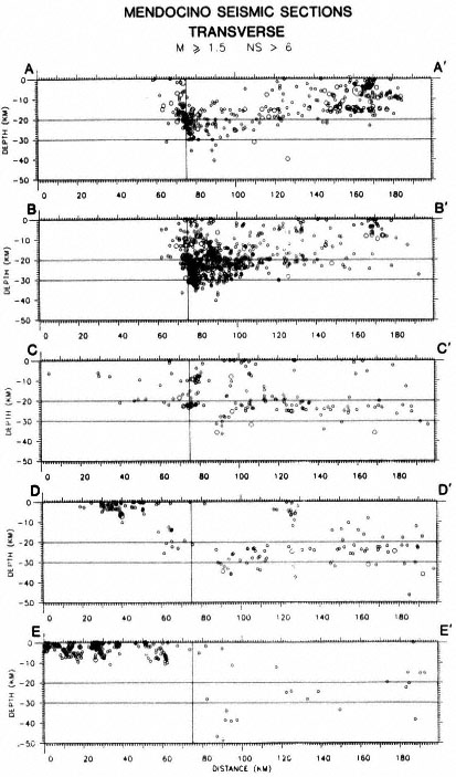
Figure 8
Transverse cross sections of the Mendocino seismic zone. Regions
corresponding to sections A–Á through E–É are outlined in figure 6. Only
earthquakes with magnitudes greater than or equal to 1.5 ( M ³ 1.5) and with
seven or more stations in the hypocentral solution ( NS > 6) were included.
only by modest clusters of events at 10- and 25-km depths, and farther east is unmarked by earthquakes.
The aftershocks of the 1980 Eureka earthquake are prominent on section A–Á at depths from the surface to about 20 km and at distances of 120 km to 180 km on the profile. The 1980 aftershock zone runs diagonally across region A–Á and passes out of it to the west at about 120 km on the profile. On section B–B́ the 1980 aftershocks are represented by the shallow cluster at 170 km. This cluster occurred about 20 km southeast of the eastern end of the principal 1980 fault break during the 1980 aftershock sequence (fig. 6).
The character of the scattered events north of the fracture zone and east of the 1980 aftershock zone appears simplest in sections C–Ć and D–D́, from 20 to 100 km east of the shoreline. On C–Ć these earthquakes appear to occur largely in a 100-km-thick zone between 20 and 30 km deep. This zone is horizontal between about 130 and 190 km on the profile. It appears to bow upward between 95 and 130 km and to bend downward sharply south of 95 km just before an abrupt cutoff at 85 km. In section D–D́ the zone is slightly thicker and more uniform in depth, although it does bend downward at its south end between 90 and 100 km on the profile. In section E–É events of this group are sparser than farther west and appear primarily in three patches: 80 to 100 km, 120 to 150 km, and 170 to 190 km. The patch on the south, at about 90 km, descends to a depth of about 50 km. A west-northwest to east-southeast profile through the zone of scattered earthquakes suggests that the zone dips very gently eastward for about 70 km from the coastline and then more steeply farther east. However, the number of events defining the steeply dipping part of the zone is very small (Cockerham, 1984).
The group of earthquakes discussed above is more difficult to isolate on sections A–Á and B–B́ because it merges with events along the fracture zone on the south and along the 1980 aftershocks zone on the north. On section A–Á these events appear in a horizontal band 10 to 20 km deep between 110 and 180 km on the profile. This band appears to thicken south of 110 km and to merge with events along the fracture zone at depths of 15 km to at least 30 km. On section B–B́ these events define a band 15–25 km deep between 110 and about 180 km. South of 110 km the zone thickens and appears to blend into the concentrated zone of hypocenters just north of the fracture zone. Heavier concentrations of events just north of the fracture zone suggest that the earthquakes may be related to disrupted seismogenic slab fragments. The scattered events on C–Ć at distances less than about 75 km mostly lie offshore, west of the inferred trace of the San Andreas fault. They suggest that earthquakes occur as deep as 20 km, but the network coverage is poor, and hypocentral locations are uncertain in this region.
The northern ends of the Maacama and Bartlett Springs faults appear as the shallow zones of earthquakes (0–10 km deep) between 20 and 50 km on section D–D́ and o and 65 km on section E–É. The sharp change in max-
imum depth of earthquakes marks the boundary between the Mendocino and Coast Ranges seismic zones.
Coast Ranges Seismic Zone
An expanded map of the Coast Ranges seismic zone, with outlines of regions for which cross sections were constructed, is shown in figure 9. The pattern of seismicity and its relationship to the San Andreas fault, as well as the position of the fault within the Coast Ranges, vary greatly from southeast to northwest. The most extensive feature of the seismicity is a nearly continuous band of earthquakes near the midline of the Coast Ranges, extending from Cholame on the southeast to Laytonville on the northwest. This line coincides with the creeping section of the San Andreas fault where it runs diagonally across the Coast Ranges between Cholame and Corralitos. Seismicity along the San Andreas is weak where it approaches the Coast northwest of the actively creeping section, between Corralitos and San Francisco along the southern end of the 1906 earthquake rupture zone. Northwest of San Francisco, where the 1906 offsets were largest, the San Andreas lies along the western edge of the Coast Ranges and is almost aseismic. Southeast of Cholame, in the region of the 1857 earthquake rupture zone, the San Andreas lies along the eastern edge of the Coast Ranges and, as northwest of San Francisco, is virtually aseismic.
In the region of complex faulting southeast of Hollister, adjacent to the section where creep dies out along the San Andreas, both the dense line of earthquakes and fault creep branch northward off the San Andreas fault onto the Calaveras fault farther east. The line of earthquakes follows the Calaveras, Hayward, Healdsburg, and Maacama faults, in order, past the east side of San Francisco Bay and on northwestward to Laytonville. A second, less continuous line of earthquakes branches eastward from the Calaveras fault south of Livermore. The second line can be followed northwestward from Livermore along the Greenville, Concord, Green Valley, and Bartlett Springs faults as far as Covelo. This line lies 30 to 40 km east of the principal Calaveras/Maacama line, and along its southern half it lies near the eastern edge of the Coast Ranges.
An apparent southeastward continuation of the line of earthquakes near the east edge of the Coast Ranges follows the Ortigalita fault from San Luis Reservoir to New Idria, east of the northern part of the creeping section of the San Andreas fault. An ill-defined linear zone of earthquakes west of the Coalinga/Kettleman aftershock zone suggests that the Ortigalita trend may extend even southeast of New Idria.
Additional, more prominent features of the southern part of the Coast Ranges seismic zone, however, are the broad bands of scattered earthquakes that lie along the flanks of the Coast Ranges, particularly on the eastern flank southeast of New Idria. There, the 20-km-wide by 50-km-long aftershock
Figure 9
Map of the Coast Ranges seismic zone showing regions (I–Í, A–Á, etc.)
for which cross sections were prepared. Abbreviations: SAF = San Andreas
fault, NFZ = Nacimiento fault zone, OF = Ortigalita fault, CF = Calaveras
fault, HF = Hayward fault, GF = Greenville fault, GVF = Green Valley fault,
BSF = Bartlett Springs fault, HBF = Healdsburg fault, MF = Maacama fault,
COA/ KET = Coalinga/Kettleman aftershock region.
Figure 10.
Longitudinal cross sections along the Maacama/Calaveras fault zone (I–Í)
and the San Andreas fault (II–IÍ). Only earthquakes with magnitudes
greater than, or equal to 1.5 (M ³ 1.5) and with seven or more stations
in the hypocentral solutions (NS > 6) were included. The dashed lines
mark the apparent lower limit of the zone of continuous seismicity along
the faults. The widths of the zones of earthquakes included on the plots
are 60 km for I–Í and 30 km for II–IÍ. Vertical exaggeration of these
sections is two times. Abbreviations: LV = Laytonville, CL = Clear Lake,
SB = Suisun Bay, LVM = Livermore, SF = San Francisco, COR =
Corralitos, BV = Bear Valley, PKF = Parkfield, CH = Cholame.
zone of the 1983 Coalinga and 1985 Kettleman Hills earthquakes, is the dominant feature on the map for 1980–1986. Both these large earthquakes, as well as almost all of their larger aftershocks, had thrust or reverse fault sources on planes with strikes nearly parallel to the San Andreas (Eaton, in press). The aftershock zone shows the extent of the zone of crustal shortening near Coalinga. Its large width contrasts sharply with the narrow lines of epicenters that mark creeping sections of the major near-vertical strike-slip faults and of the aftershocks of the large earthquakes that occur along them (Eaton et al., 1970; Cockerham and Eaton, 1987).
To examine the Coast Ranges seismicity in more detail, we have constructed cross sections for each of the boxes outlined on figure 9. Events within each box were projected onto a vertical plane parallel to the long axis of the box. Sections I–Í and II–IÍ (fig. 10) are longitudinal sections parallel to the dense lines of earthquakes in the northern Coast Ranges (Maacama, Bartlett Springs to Calaveras faults) and the southern Coast Ranges (San Andreas fault), respectively. The northern box (I–Í) is 60 km wide in order to include both the central and eastern lines of earthquakes, while the south-
ern box (II–IÍ) is only 30 km wide in order to separate activity on the San Andreas from that on its major branches north of Hollister.
The longitudinal profiles illustrate two principal aspects of seismicity along the faults: (1) the intensity of seismic activity along the fault and (2) the depth to the bottom of the continuous seismogenic zone along the fault. Two reference lines are drawn on the longitudinal sections. The first is a straight line at 15-km depth. The second (dashed) line marks the depth of the abrupt decrease in the abundance of earthquakes at the apparent base of the continuous seismogenic zone. Some of the scattered hypocenters below this line are reliably located and deserve special note. Others are possibly poorly located events that occurred at shallower depths.
Earthquakes on profile I–Í are moderate in number and rather evenly distributed along the fault from Laytonville to Suisun Bay (0 to 250 km) except for the dense shallow cluster of events in the Geysers/Clear Lake region (135 to 155 km). The depth to the bottom of the continuous seismogenic zone averages about 10 km over this region. It descends to about 12–13 km south of the Geysers/Clear Lake region and rises to only 5 km beneath, and just north of, that region. A small deeper cluster of well-located events, however, lies at 13–18 km beneath the shallow continuous seismogenic zone near Clear Lake. Near Suisun Bay the eastern line of seismicity lies at the eastern edge of the Coast Ranges, and earthquakes beneath Suisun Bay occur as deep as 15–25 km. Farther southeast along profile I–Í the bottom of the seismogenic zone ranges between 10 and 15 km and averages 12 to 13 km deep. The heavy concentration of events along this southern section of the profile reflects both an increased level of background seismicity and aftershocks of several large earthquakes.
The most prominent feature on section II–IÍ is concentration of earthquakes along the creeping section of the San Andreas fault, between Corralitos (120 km) and Parkfield (280 km). The base of the continuous seismogenic zone ranges from 10 to 15 km and averages 12 to 13 km deep along this section. Northwest of Corralitos, between 90 and 120 km on the profile, earthquakes shallower than 10 km are virtually absent, although weak seismicity between 10 and 15 km deep continues beneath the quiet zone. Farther northwest, patches of small, infrequent earthquakes occur between the surface and about 12 km deep in the distance ranges 55 to 90 km and 5 to 35 km. The northernmost of these earthquakes are on the San Andreas fault adjacent to San Francisco.
Seismicity along most of the southern half of the actively creeping section of the San Andreas, between about 210 and 256 km on the profile, is less intense than along the northern half (120 to 210 km) and at the extreme southern end just north of Parkfield. Most events in this section of less intense seismicity are between 2 and 12 km deep. The section of the fault that
broke in the 1966 Parkfield earthquake, between about 280 and 320 km on the profile, is less seismic than the section northwest of Parkfield, and earthquakes along this section die out southeastward. Southeast of Cholame (320 km) there is a 10-km gap in seismicity followed by weak seismicity between 330 and 360 km. This southeasternmost patch of earthquakes on the profile is mostly between 8 and 15 km deep.
The transverse sections A–Á to D–D́ in figure 11 were positioned to illustrate how the pattern of seismicity transverse to the Coast Ranges varies along their length. Each section is 200 km long and shows earthquakes from an 80-km wide box across the Coast Ranges projected onto a vertical plane that is perpendicular to the dense line of earthquakes traversing the box. On these sections, strike-slip faults perpendicular to the boxes appear as narrow, near-vertical linear concentrations of events. On all four sections the vertical line of events near 100 km on the profile represents the most prominent line of epicenters (fig. 9) near the midline of the Coast Ranges. It represents the San Andreas fault on D–D́, the Hayward fault on C–Ć, the Healdsburg fault on B–B́, and the Maacama fault on A–Á. The vertical lines of events at 130 to 140 km on profiles A–Á, B–B́, and C–Ć represent the line of epicenters, about 35 km east of the midline, along the eastern edge of the Coast Ranges. In section D–D́ the great mass of events between about 125 and 145 km represents the aftershocks of the 1983 Coalinga and 1985 Kettleman Hills earthquakes athwart the boundary between the Coast Ranges and the Great Valley.
South-to-north variations in seismicity of the San Andreas are demonstrated dramatically by the cross sections. Earthquakes along the southern 80 km of the creeping section of the San Andreas are densely clustered in a vertical line from the surface to a depth of about 13 km (D–D́). Earthquakes on the San Andreas near San Francisco are few in number and scattered over a somewhat broader zone than farther south (C–Ć). Section B–B́ north of San Francisco shows the San Andreas to be virtually aseismic. Section A–Á from Point Arena northward shows only minor seismicity along the San Andreas.
Most of the deeper earthquakes on the cross sections occur beneath the Great Valley or near the eastern boundary of the Coast Ranges. On section B–B́ the events 10 to 20 km deep near 190 km on the profile occurred about 10 km east of the Coast Ranges boundary, 20 km southwest of the Sutter Buttes. On section C–Ć the sparse, vertically elongated zone of earthquakes 15 to 25 km deep between 130 and 140 km on the profile is beneath Suisun Bay where the Valley indents the eastern edge of the Coast Ranges. On section D–D́ the earthquakes deeper than 15 km mostly lie beneath and east of the Coalinga/Kettleman aftershock zone. Although relatively few in number (about one percent as many as the Coalinga/Kettleman aftershocks), these
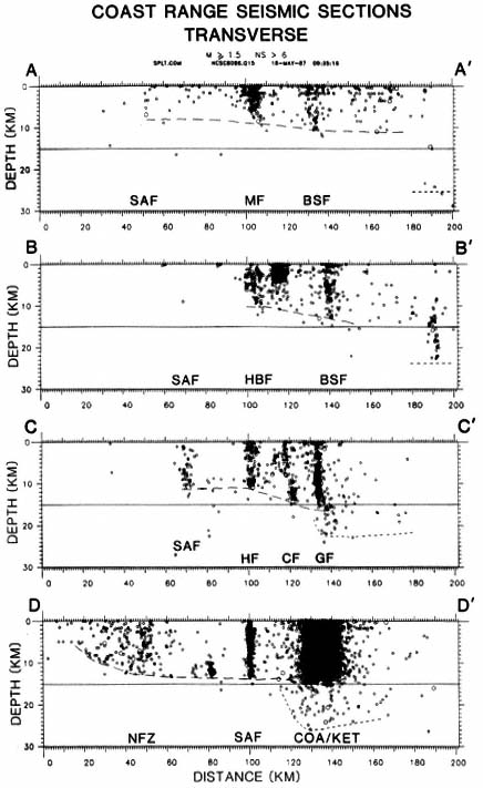
Figure 11
Tranverse cross sections of the Coast Ranges seismic zone. The regions
projected onto profiles A–Á through D–D́ are outlined in figure 9. Each
profile is centered on, and perpendicular to, the continuous line of
earthquakes near the Coast Ranges midline. Dashed lines indicate the
approximate bottom of the seismogenic zone beneath the Coast Ranges.
The events deeper than 15 km on the right end of the profiles are beneath
the eastern edge of the Coast Ranges or the adjacent Great Valley. The
dotted line indicates the approximate bottom of the seismogenic zone
beneath the Coast Ranges/Great Valley boundary region. Two times
vertical exaggeration. Abbreviations as for figure 9.
events cannot be ascribed to poor locations, and they reveal a broad zone of mild seismicity in the lower crust beneath the eastern edge of the Coast Ranges and adjacent Great Valley.
On sections A–Á to C–Ć the San Andreas fault lies near the coastline and the continental margin. On D–D́ it is about 70 km inland, and seismicity in the Coast Ranges west of the fault is remarkably different from that west of the fault, offshore on the northern cross sections. A landward-thickening zone of diffuse seismicity extends inland from the west end of the profile to near 60 km on the profile. The zone of modest concentration of events near 50 km corresponds approximately to the Nacimiento fault. Except for a concentrated cluster of events 10 to 13 km deep near 80 km on the profile (San Ardo), there is little seismicity between about 65 and about 100 km (San Andreas fault). The lower limit of the seismic zone is very sharp from about 10 km, where it is about 5 km deep, to the San Andreas, where it is about 13 km deep. Crustal seismicity is weak for about 15 km northeast of the San Andreas. Farther east, but still west of the Coalinga/Kettleman aftershocks, the density of earthquakes in the upper crust increases moderately, and earthquakes appear in the lower crust. Focal mechanisms of large earthquakes in the bands of seismicity along the coast, as well as in the Coalinga/ Kettleman region, show that both flanks of the Coast Ranges in box D–D́ are under compression normal to the San Andreas fault, and that the predominant mode of failure is along thrust and reverse faults on planes with strikes parallel to the San Andreas (Eaton, 1985; Eaton and Rymer, in press).
Tectonic Implications
Global plate tectonics provides an overview of the relative motion of the North American, Pacific, and Gorda/Juan de Fucca plates along their common boundaries in northern California: the San Andreas fault, the Mendocino fracture zone, and the coastal subduction zone north of Cape Mendocino. Plate tectonics studies, however, tell us little about the structure of the boundaries. Detailed local observations are needed to define particular
boundaries more precisely and to study the processes in the crust and upper mantle through which they operate.
Contemporary seismicity provides a snapshot of the number, location, size, and style of faulting associated with the plate boundaries and the triple junction. The record of seismicity based on instrumental studies is incomplete because of its short duration, but it can be supplemented by the longer-term historical seismic record. Earthquakes are important symptoms of deformation of the Earth's crust and mantle, but tell only part of the story. Much deformation occurs silently, particularly in the mantle and lower crust. This limitation must be kept in mind when we use seismicity to infer processes in the crust. Nonetheless, the northern California seismicity data do document the generation of earthquakes by plate boundary processes over a very large region with remarkable uniformity and sensitivity. The mechanical implications of the seismicity data, as well as their sensitivity and areal extent, invite their use to compare and contrast crustal processes in the two major seismic regions of northern California, the Mendocino and Coast Ranges seismic zones.
Mendocino
The pattern of earthquakes in the Mendocino seismic zone suggests that the southeastern corner of the relatively young and weak Gorda plate is being crushed against the northeastern corner of the older, stronger Pacific plate in consequence of the convergent component of relative motion in the region. The larger right-lateral strike-slip component of relative motion should carry the disrupted remnants of the south edge of the Gorda plate eastward beyond the east edge of the Pacific plate, where these remnants appear to be obducted onto (or against) the western edge of the North American plate. Subsequent northwestward motion of the Pacific plate relative to the North American plate should entrain the Gorda-plate debris in the boundary zone between those plates in the northern Coast Ranges.
The continuity of the grossly furrowed topography onshore between Cape Mendocino and Trinidad Head with that east of the Maacama fault farther south suggests that these regions share important features of origin and internal structure. The Franciscan Complex, which largely coincides with that topography, contains much material that appears to have been crushed and mixed by a process like that now affecting the southeastern corner of the Gorda plate (Fox, 1983a ).
The present geometry of the Gorda ridge relative to the Blanco fracture zone on the north and the Mendocino fracture zone on the south suggests that the southern quarter of the ridge, where it curves to remain perpendicular to the Mendocino fracture zone, is becoming inactive and is requiring an adjustment in the location of the Mendocino fracture zone between the Gorda ridge and the Mendocino triple junction. Such a readjustment is also
suggested by the trend of the band of earthquakes along the fracture zone just west of Cape Mendocino. The torque required to rotate the Gorda/Juan de Fuca plate in a clockwise direction and to maintain the plate-crushing contact between the Gorda and Pacific plates just west of Cape Mendocino, may be produced by the southeastward drag along the eastern edge of the Gorda plate caused by its oblique subduction beneath the North American plate. Left-lateral faulting on northeast striking faults across the southeastern corner of the Gorda plate (Silver, 1971 ), such as occurred during the November 8, 1980, earthquake, is a consequence of the strong normal forces developed across the eastern end of the Mendocino fracture zone by the process outlined above.
Coast Ranges
The driving force behind earthquakes in the Coast Ranges seismic zone is the transform (boundary) between the North American and Pacific plates. Details of the gross physical properties of this boundary and how it works are lacking. Some outstanding questions are: (1) How wide is the transform in the upper mantle, and where is it located relative to the San Andreas fault and the midline of the Coast Ranges? (2) Is displacement across the transform in the mantle abrupt and discontinuous, as at a fault, or distributed in some manner across a broad zone? (3) Is the upper crust decoupled from the lower crust and upper mantle over the transform? (4) Do rigid sections of the upper crust resist internal deformation and "integrate" distributed displacement across their bases and concentrate it in faults along their edges?
The principal observations from contemporary seismicity and the historical seismic record can be summarized by the following statements: (1) The maps and cross sections presented above show that the Coast Ranges seismic zone is complex and that its most prominent features vary from northwest to southeast within it. (2) Most of the displacement between the Pacific and North American plates at the Earth's surface occurs on the San Andreas fault. (3) Where the San Andreas crosses the center of the Coast Ranges, between Cholame and Corralitos, most of the displacement occurs as creep accompanied by countless small earthquakes; where it lies along the edges of the Coast Ranges most of the offset occurs during infrequent, very large earthquakes. (4) Long-term offset rates (over hundreds of years) across the Calaveras/Maacama and Greenville/Bartlett Springs fault zones, which are marked by linear concentrations of small earthquakes like that along the rapidly creeping section of the San Andreas, are small compared to that on the San Andreas (now locked) farther west. (5) The trace of the San Andreas fault between Point Arena and Cape Mendocino lies offshore and is difficult to identify. It is believed to deflect about 40 km to the east and generally to follow the coast north of Point Arena. Macroseismic effects of the 1906 earthquake indicate that this northernmost section of the fault broke in 1906. The
long-term offset rate on this section should be the same as that south of Point Arena, but the total offset across it should decrease to zero as it approaches the triple junction, which is its point of origin. (6) The depth to the base of the seismogenic zone along the principal strike-slip faults in the Coast Ranges averages about 10 km north and 12 to 13 km south of Clear Lake. The depth to the base of the seismogenic zone appears to increase gradually from west to east across the Coast Ranges. This effect is most pronounced along the eastern margin of the Coast Ranges and the adjacent Great Valley, where focal depths are as great as 15 to 25 km. Earthquakes deeper than 15 km (in the lower crust) are extremely rare elsewhere in the Coast Ranges but common beneath the Great Valley. (7) Both flanks of the Coast Ranges southeast of Hollister are marked by scattered patches and broad zones of earthquakes whose sources indicate crustal compression normal to the San Andreas fault. These earthquakes may be caused by lateral spreading of the southern Coast Ranges resulting from misalignment between the San Andreas fault in the upper crust and a more northerly trending transform in the mantle below. Such a misalignment is suggested by recent studies of global plate-motion directions (Minster and Jordan, 1984).
From the distribution of current seismicity and the position of the San Andreas fault, it appears that the entire Coast Ranges is underlain by a broad zone of right-lateral shear deformation. The restriction of earthquakes to the upper crust beneath the Coast Ranges, but not beneath the contiguous portions of the Great Valley on the east or the Mendocino seismic zone on the north, suggests that the lower crust deforms plastically beneath at least the central part of the Coast Ranges. The branching and spacing of major strike-slip faults in the upper crust north of Hollister suggest some sort of decoupling between the brittle upper crust and the plastic lower crust. The parallel, subequally spaced traces of the three major branches northwest of Livermore suggest that sections of the brittle upper crust resist internal deformation and concentrate distributed displacements beneath them onto their fault boundaries.
Decoupling of the upper and lower crust in the southern Coast Ranges can also account for the relatively aseismic zones lying between the actively creeping San Andreas fault and the zones of compression and reverse-fault earthquakes along both the east and west flanks of the Ranges. Horizontal decoupling horizons 12 to 15 km deep beneath the center of the Ranges curve upward through the brittle upper crust where it is driven beyond the margins of the plastic zone (over the transform) in the lower crust (Eaton and Rymer, in press).
Evidence for tracing the San Andreas between Point Arena and the triple junction is very weak. The principal zone of displacement between the Pacific and North American plates most likely lies near the coastline just southeast of the triple junction: the intense zone of seismicity between the
Gorda and Pacific plates terminates abruptly where the Mendocino fracture zone intersects the coastline. Farther south, the trace of the San Andreas is well defined where it strikes northwestward out to sea just north of Point Arena. Here, its trace is subparallel to, but offset about 40 km to the southwest of, the coastline southeast of Cape Mendocino. The most prominent feature of the rather weak seismicity linking these two sections of the fault is the diffuse north-south trending band of small earthquakes between Point Arena and the northern end of the line of earthquakes along the Maacama fault (fig. 5). The offset of the San Andreas may be associated with this band of earthquakes.
The sliver of crust between the Calaveras/Hayward/Maacama and San Andreas faults is an enigma. Its eastern boundary is marked by the line of frequent small earthquakes along the Coast Ranges midline, and its western boundary is the virtually aseismic section of the San Andreas that produced the 1906 earthquakes. South of Clear Lake it is nearly aseismic, but north of Clear Lake it contains diffuse clusters of small earthquakes. Topographically, this region is much simpler and more homogeneous than the region just east of the Calaveras/Maacama fault zone, which is characterized by bold northwest trending ridges of such relief and length as to suggest a tectonic origin (Fox, 1983b ). These relationships suggest a marked difference in the response of the upper crust west and east of the Calaveras/Maacama fault zone to the right-lateral strain across the Coast Ranges. West of that zone, the upper crust stores accumulating strain, without internal disruption, for eventual release along the San Andreas in a major earthquake. Along and east of that zone, it appears to yield gradually by internal deformation and slip along boundaries within it in a manner that may limit the size of earthquakes it can produce and enhance the grossly ridged topography that characterizes it.
References
Atwater, Tanya (1970). Implications of plate tectonics for the Cenozoic tectonic evolution of western North America. Geol. Soc. Am. Bull., 81: 3513–3536.
Bolt, B. A., C. Lomnitz, and T. V. McEvilly (1968). Seismological evidence on the tectonics of central and northern California and the Mendocino Escarpment. Bull. Seism. Soc. Am., 58: 1725–1767.
Bolt, B. A., and Roy D. Miller (1975). Catalog of Earthquakes in Northern California and Adjoining Areas: 1 January 1910–31 December 1972. Seismographic Stations, University of California, Berkeley, 1–567.
Cockerham, R. S. (1984). Evidence for a 180-km-long subducted slab beneath northern California. Bull. Seism. Soc. Am., 74: 569–576.
Cockerham. R. S., and J. P. Eaton (1987). The earthquake and its aftershocks, April 24 through September 30, 1984. In Seena N. Hoose, ed., The Morgan Hill, California, earthquake of April 24, 1984. U.S. Geol. Surv. Bull. 1639, 15–28.
Eaton, J. P. (1981). Detailed study of the November 8, 1980 Eureka, California,
earthquake and its aftershocks (abs.). EOS, 62: 959.
——— (1985). The May 2, 1983 Coalinga earthquake and its aftershocks: A detailed study of the hypocentral distribution and of the focal mechanisms of the larger aftershocks. In M. J. Rymer and W. L. Ellsworth, eds., Mechanics of the May 2, 1983 Coalinga Earthquake. U.S. Geol. Surv. Open-file Report 85–44, 132–201. Menlo Park, California. Regional seismic background of the May 2, 1983 Coalinga earthquake. Op. cit., 44–60.
Eaton, J. P., W. H. K. Lee, and L. C. Pakiser (1970). Use of microearthquakes in the study of the mechanics of earthquake generation along the San Andreas fault in central California. Tectonophysics, 9: 259–282.
Eaton, J. P., and M. J. Rymer (in press). Regional seismotectonic model for the southern Coast Ranges. In M. J. Rymer and W. L. Ellsworth, eds., Mechanics of the May 2, 1983, Coalinga earthquake. U.S. Geol. Surv. Professional Paper 1487.
Fox, K. F., Jr. (1983a ). Melanges and their bearing on late Mesozoic and Tertiary subduction and interplate translation of the west edge of the North American plate. U.S. Geol. Surv. Professional Paper 1198, 1–40.
——— (1983b ). Tectonic setting of late Miocene, Pliocene, and Pleistocene rocks in part of the Coast Ranges north of San Francisco, California. U.S. Geol. Surv. Professional Paper 1239, 1–33.
Jennings, C. W., compiler (1975). California Data Map No. 1: Faults, Volcanoes, and Thermal Springs and Wells. California Divisior of Mines and Geology.
Minster, J. B., and T. H. Jordan (1984). Vector constraints on Quaternary deformation of the western United States east and west of the San Andreas fault. Pacific Section Soc. Econ. Paleontology and Mineralogy, 38: 1–16.
Silver, E. A. (1971). Tectonics of the Mendocino triple junction. Geol. Soc. Am. Bull. 82: 2965–2978.
Fourteen—
Hypocenter Mapping and the Extensibility of Seismotectonic Paradigms
James W. Dewey
Introduction
This paper will consider earthquake mapping from the viewpoint of scientific "paradigms," in the context of Kuhn's (1970) theory of the structure of scientific revolutions. Paradigms are "universally recognized scientific achievements that for a time provide model problems and solutions to a community of users" (Kuhn, 1970, p. viii ). A paradigm is a framework within which the community identifies and solves the puzzles of its discipline. It provides both a basis for interpreting old data and, more important in the long run, a rationale for acquiring new data. A paradigm may be gradually modified in order to account for new results of ongoing observations. From time to time, the community may face observations that either contradict the paradigm in a fundamental way or that are both inexplicable by the paradigm and too important for the community to ignore. The community ultimately resolves such a crisis by adopting a radically new paradigm that accounts for the observations that led to the old paradigm and that also explains the observations that could not be accounted for by the old paradigm. This radical change of paradigm, in Kuhn's model, constitutes a scientific revolution.
For the past two decades, most research in seismotectonics has been based on two paradigms. On a local scale, we have the earthquake/fault paradigm: societally and tectonically significant crustal earthquakes commonly occur as the result of shear displacement on preexisting geologic faults that are big enough to, in principle, be imaged by appropriate geologic or geophysical data. On a broad scale, there is what I will call the earthquake/plate-tectonics paradigm: the locations and focal mechanisms of many earthquakes are predictable from a knowledge of the relative motions of tectonic plates on the Earth's surface and by application of a few simple constitutive rules governing plate behavior. Seismotectonic research is commonly based on both
paradigms, but this is not always so. I find it convenient from an expository standpoint to consider the two paradigms separately.
At present, neither the earthquake/fault nor earthquake/plate-tectonics paradigm faces anomalies of the sort that imply an imminent revolution throughout seismotectonics. There are, however, some earthquake source regions that have been studied from the viewpoints of the two paradigms and that nevertheless remain poorly understood. Seismicity data from these regions do not strongly suggest slip on preexisting faults when interpreted by the current fault paradigm, or the working of a particular plate-tectonics process when interpreted by the current plate-tectonics paradigm. Moreover, there is a precedent for proposing locally applicable models that are essentially independent of the current earthquake/fault and earthquake/plate-tectonics paradigms. Individual earthquakes have, for example, been modeled as consequences of large landslides (Kanamori et al., 1984; Eissler and Kanamori, 1987) or of tensile failure under high fluid pressure (Julian, 1983). Seismologists who work in puzzling source regions therefore face three options. They can continue to apply current plate-tectonics and fault paradigms, hoping that more and higher quality data will reveal the nature of the source regions. Alternatively, they can try to explain the existing observations by modifying the current paradigms without abandoning the fundamental assumptions upon which the paradigms are based. Finally, they can abandon the paradigms altogether and, hoping to precipitate a scientific revolution in a subfield of seismotectonics, search for locally applicable seismotectonic models that do not involve plate-tectonics processes or slip on preexisting faults.
This paper will attempt to demonstrate the value of the two conservative options for solving local puzzles—the collection of more data in the framework of existing paradigms and the elaboration of existing paradigms. My intent is not to belittle the importance of contemplating radically new paradigms but rather to convey the extent to which recent observational studies and recent elaborations have strengthened the existing paradigms. A wide range of phenomena is already at least partially accounted for by the paradigms; the solution to some local puzzles may lie in a few more data points plus the application of hypotheses developed in other seismic zones. Furthermore, the paradigms have continued to be extensible to cover previously unexplained observations and are therefore likely to be extensible in the future to cover still more observations.
The Earthquake/Fault Paradigm
The hypothesis that earthquakes result from faulting developed near the turn of the century (Dutton, 1904; Reid, 1910) and evolved with contributions from many scientific disciplines. Although different communities of earth sci-
entists have different studies of seismogenic faulting as models, and their paradigms accordingly differ somewhat, I would suggest that the basic earthquake/fault paradigm for mapping crustal shocks comprises the following theses: (1) most crustal earthquakes result from the release of tectonic strain energy by sudden shear fracture along preexisting faults; (2) high-quality seismicity data from an active crustal source region will define two-dimensional planar or slightly curved zones of hypocenters, corresponding to faults, and focal mechanisms will have nodal planes parallel to the local orientations of the hypocentral surfaces; and (3) large crustal earthquakes occur on large faults, which therefore may extend from seismogenic depths to the near-surface and be mappable with geologic or geophysical data. The preceding theses are hypotheses and expectations that appear inherent in the ways in which observational seismologists design seismicity studies and in the ways in which they seem most naturally to interpret the resulting hypocenters and focal mechanisms.
A suite of observations that exemplify each of the theses in the basic earthquake/fault paradigm is found in the Parkfield, California, section of the San Andreas fault (fig. 1). Five earthquakes of magnitude about 6 have taken place since 1857 on apparently the same segment of the fault; the coseismic displacement seismologically inferred for each shock appears equal to the displacement that would be expected to accumulate elastically across the fault between shocks (Bakun and McEvilly, 1984). The most recent such shock occurred in 1966; geodetic data are consistent with the segment of fault that ruptured in 1966 being currently locked at depth and accumulating strain (Harris and Segall, 1987). Small and moderate earthquakes occur on a nearly vertical plane beneath the surface trace of the fault and have mechanisms consistent with slip on the fault. The fault zone is conspicuous in regional geology and geomorphology.
In a region in which seismogenic faults are not revealed in seismographic or geologic data as directly as the San Andreas fault is revealed near Parkfield, the earthquake/fault paradigm may be elaborated as in studies of the Coalinga earthquake of 2 May 1983 (fig. 1). Hypocenters and focal mechanisms in the Coalinga region do not define a single plane, and the causative fault of the main shock of 2 May 1983 does not outcrop at the surface. The hypocenters and focal mechanisms are, however, well accounted for in terms of slip on intersecting faults (Eaton, 1985b ). Stein and King (1984) have shown that the seismogenic reverse or thrust faulting that occurred at depth appears to manifest itself as folding in the weak near-surface sedimentary rock. They suggest that, in regions in which surface rock is sedimentary, the presence of reverse faulting at depth may often be found more easily by searching for associated folds rather than outcrops of fault planes. In this case, the apparent failure of the Coalinga earthquake to conform to the third thesis of the earthquake/fault paradigm led to a richer version of the para-
Figure 1
Seismicity of central California in the region of Parkfield and Coalinga
for the period 1975–1984 (from Dewey et al., in press, after Bakun and
Lindh, 1985). Focal mechanisms of the 1966 Parkfield and 1983 Coalinga
earthquakes are shown. N35° W is the direction of pure transform motion
between the Pacific and North American plates.
digm, in which active surface folds are added to active fault traces as possible indicators of potentially dangerous earthquake sources.
The seismicity of central Idaho (fig. 2) provides examples of several phenomena not yet, but probably soon to be, incorporated into the earthquake/fault paradigm. These phenomena are the quiescence of major faults at the small magnitude level for long periods between the generation of large earthquakes, the occurrence of small and moderate earthquakes away from major faults, and the occurrence of aftershocks on faults other than those of the corresponding main shocks.
Central Idaho was the site of the magnitude (Ms ) 7.3 Borah Peak earthquake of 28 October 1983. The cause of that earthquake was slip on a major preexisting fault, the Lost River fault (Crone et al., 1987), most of which had been quiescent down to magnitude 3.5 during the previous two decades (fig. 2). From 1963 until the 1983 Borah Peak main shock, small and moderate earthquakes in central Idaho had occurred most frequently several tens of kilometers west and north of the Borah Peak source. Although aftershocks in the first ten days following the main shock were located close to the coseismic fault surface defined from geologic and geodetic data, later aftershocks occurred in a zone twice as long as the main-shock rupture (fig. 2).
Such observations might be viewed as already accounted for in an extended earthquake/fault paradigm, because they are considered possible outcomes of seismicity studies premised on the seismogenic-fault model. But I am not aware of an independently defined community of users that has reached consensus about the seismotectonic environments in which these phenomena should be considered expected outcomes of seismicity studies.
The phenomenon of fault quiescence is currently being studied using the hypothesis that individual segments of seismogenic faults slip by characteristic amounts in the coseismic phase of each seismic cycle, and that the characteristic displacement and interval between displacements of a given fault segment tend to increase with segment length (Allen, 1968, Sieh, 1978; Schwartz and Coppersmith, 1984). Faults that comprise many segments are most likely to experience frequent small and moderate shocks; faults that comprise a few large segments are most prone to long periods of quiescence separated by large earthquakes. This characteristic-displacement hypothesis would lead to an elaboration of thesis 2 of the earthquake/fault paradigm. Although seismographic recording in active source regions would still be expected to define planar faults, the largest faults in the region might not be revealed in a time period much shorter than the durations of the seismic cycles on the faults. Quiescence at small and moderate magnitudes would be expected in a short period of seismographic monitoring of a fault if geologic studies showed the fault to be geometrically simple with a recent history of large, episodic displacements.
The characteristic-displacement hypothesis also explains the observation
Figure 2
Seismicity of central Idaho in the vicinity of the Borah Peak earthquake of 28 October
1983. Epicenters are distinguished according to whether the shocks occurred before,
within ten days after, or between ten days and two years after the Borah Peak main
shock. Epicenters were computed by Dewey (1987). Borah Peak fault scarps are from
Crone et al. (1987), and the rupture surface is from Ward and Barrientos (1986).
that some large earthquakes are followed by aftershocks near, but not on, the main-shock rupture surface. Stress is effectively relaxed on the simple main-shock source by the occurrence of the main shock, and most of the main-shock surface will not rupture again until sufficient strain energy has accumulated to again produce the characteristic displacement. Aftershocks occur on the margins of the main-shock rupture, due perhaps to slip on smaller branch faults, which must accommodate some of the displacement of the main fault (King, 1983), or to slip on preexisting faults on which effective shear stress has increased as a consequence of main-shock faulting (Chinnery, 1966; Nur and Booker, 1972). Many aftershock studies are conducted on the assumption that aftershock hypocenters are distributed on the surface that slipped in the main shock. Under the characteristic-displacement hypothesis applied to aftershock sequences, the location of aftershocks of a major earthquake would be expected to define fault surfaces secondary to the fault surfaces on which most of the main-shock seismic moment was released.
Small earthquakes occurring kilometers to tens of kilometers away from major regional faults have traditionally been interpreted as due to minor faults slipping under the same regional tectonic stress causing slip on the major faults (Richter, 1958). Substantial elaboration of this interpretation has come with studies showing the wide range of preexisting fault orientations that may be favorable to slip under a given stress field (McKenzie, 1969; Angelier, 1984). It is also commonly accepted that some small earthquakes may reflect local stress fields that are either independent of the regional stress field or second-order consequences of large tectonic displacements induced by the regional stress field. Algorithms have been developed that permit extraction of several significantly different orientations of focal mechanisms from a suite of first motion data for a group of earthquakes (Brillinger et al., 1980) and that enable a search for a single orientation of the tectonic stress field that may be consistent with differently oriented focal mechanisms (Gephart and Forsyth, 1984).
Midplate regions, located far from the belts of earthquakes and late-Cenozoic deformation that define plate boundaries in the earthquake/plate-tectonic paradigm (see next section), pose special problems for the earthquake/fault paradigm. In most midplate areas monitored by regional or local networks of seismographs, the resulting hypocenters and focal mechanisms do not define planes of shear displacement coinciding with mapped crustal faults (for example, see Bollinger and Sibol, 1985; Wetmiller et al., 1984). It is possible that, in some of these areas, midplate earthquakes do not occur on preexisting faults but rather represent fractures of previously intact rock, being thereby natural analogs of some mine rockbursts (Evernden, 1975). In that case, the distribution of microcracks or the rheological properties of the unfractured rock, rather than the presence of geologically mappable faults, might determine the positions of earthquakes (McGarr et al.,
1975). Even if the resulting earthquakes involved the development of faults in previously intact rock, such earthquakes would not fulfill all of the expectations of the earthquake/fault paradigm. Earth scientists would lose one of the most important pratical consequences of the paradigm, that sites of future earthquakes are in principle identifiable by mapping of the faults on which they will occur. The apparent ineffectiveness of the paradigm in many midplate regions may, however, be due to the small sizes of the shocks for which the paradigm is being called upon to account. As just noted, even in areas with well-documented seismogenic faulting in the western United States, it may be difficult to associate many small earthquakes with individual faults. But in the active parts of the western United States, seismologists' confidence in the earthquake/fault paradigm does not depend on its making sense of the small shocks.
An observation that supports the appropriateness of the earthquake/fault paradigm for at least some midplate regions is that late Cenozoic reactivation of pre-Cenozoic faults has been identified at a number of sites in the central and eastern United States (Wentworth and Mergner-Keefer, 1983; Donovan et al., 1983). Most of these faults have been quiescent during the time period in which earthquakes might have been reliably located in their vicinities, but, as noted earlier in this section, quiescence of potentially seismogenic faults is quite commonly observed in regions of high Cenozoic tectonism. The crucial implication of the reactivation is that crustal faults can persist as sites of shear failure in tectonic environments that are far different from the environments in which the faults originally formed.
Results from a multidisciplinary investigation of the Mississippi Embayment seismic zone (fig. 3) have shown the value of the earthquake/fault paradigm in an important midplate seismic region. In addition, the Mississippi Embayment studies must be viewed as justifying the patience-trying accumulation of seismographic, geophysical, and geologic observations to solve a seismotectonic puzzle. The Mississippi Embayment source produced the New Madrid earthquakes of 1811 and 1812, the largest in the history of the central and eastern United States. The status of our knowledge of the distribution of earthquake epicenters in the Mississippi Embayment prior to mid-1974 is shown in the left panel of figure 3; the distribution does not suggest the presence of faults. In mid-1974, Saint Louis University installed a regional network in the Mississippi Embayment region (Stauder et al., 1976). This network greatly increased the number and accuracy of earthquake hypocenters in the Mississippi Embayment (right panel, fig. 3); the 1975–1985 data also permitted more accurate determination of hypocenters of pre-1975 shocks (Gordon, 1983). Geophysical studies conducted in the late 1970s and early 1980s suggested that the Mississippi Embayment is underlain by a late Precambrian–early Paleozoic rift (Hildenbrand, 1985), and geologic studies identified the late-Holocene Lake County uplift above the
Figure 3
Two views of seismicity of the Mississippi Embayment. At left, a pre-1975 view based on epicenters
routinely determined by the U.S. Geological Survey and its predecessors and published in catalogs such
as the "Preliminary Determination of Epicenters" (PDE). At right, a view based on epicenters recorded by
the St. Louis University Mississippi Embayment Network for 1975–1985 (small diagonal crosses) and on
pre-1975 earthquakes whose locations have been recomputed using calibration events from the post-1975
era (Gordon, 1983). The rift boundaries and outline of the Lake County Uplift, though plotted in the left
frame, are taken from the post-1975 work of Hildenbrand (1985) and Russ (1982).
most active part of the seismic zone. Epicenters, Paleozoic structure, and Quaternary data now fit a fault model quite nicely. The lineations suggested by recently recorded epicenters would correspond to individual faults being reactivated under a uniform stress system (Russ, 1982); focal mechanisms of the larger shocks of the past decade are consistent with this interpretation (Herrmann and Canas, 1978). The Lake County uplift probably represents the surface expression of a basement reverse fault (Russ, 1982; Nicholson et al., 1984) similar to the anticline that represents the surface effect of the reverse-slip fault at Coalinga, California.
The Earthquake/Plate-Tectonics Paradigm
The earthquake/plate-tectonics paradigm emerged as one aspect of the global-tectonics revolution of the 1960s (Isacks et al., 1968). According to the paradigm, the Earth's crust and upper mantle comprise continent-sized slabs, or plates, of lithosphere that move with respect to each other and that are separated by boundaries along which their relative motions are accommodated. Over geologic time, the motions of the plates relative to each other are so much greater than their internal deformations that the plates are treated as rigid in global kinematic analysis of lithospheric displacements. Earthquakes occur on the plate boundaries. The type of displacement—normal, reverse, or strike-slip—producing the earthquakes on a given boundary depends on whether the relative motion of the adjacent plates is away from, toward, or parallel to the boundary.
An example of one type of refinement of the earthquake/plate-tectonics paradigm is given by ongoing studies of the ratio of seismic to aseismic slip across a plate boundary. Plate-tectonics models can predict the amount of relative motion between two plates that must be accommodated by some kind of slip on their mutual boundary, but the original earthquake/plate-tectonics paradigm did not provide a basis for estimating the percentage of relative plate motion across a particular boundary that would be accommodated by seismic slip. Recent studies have searched for systematic dependencies of this ratio on such plate-tectonics parameters as plate age and convergence rate (for example, Kanamori, 1986).
In the United States, the dependence of the seismic/aseismic ratio on plate age is at the heart of a controversy on the likelihood of great earthquakes in the Pacific Northwest subduction zone. The kinematics of global plate motions implies a convergence of 30 to 40 mm/year across the Pacific Northwest subduction zone. The thrust interface between the Juan de Fuca and North American plates has not, however, been seismogenic during the period in which it has been instrumentally monitored. Because the Pacific Northwest subduction zone involves the subduction of young oceanic plate, and because there is a worldwide tendency for the seismic/aseismic ratio to
increase as the age of subducting lithosphere decreases, it has been suggested that the plate interface is only temporarily quiescent and is storing energy for a future great earthquake (Heaton and Kanamori, 1984). But it is not clear if the tendency for seismogenic subduction of young lithosphere can be extrapolated to imply that the very young sediment-covered lithosphere of the Juan de Fuca plate should be seismogenic. Possibly underthrusting in the Pacific Northwest is accommodated aseismically, as would be suggested by extrapolation from the recent lack of plate interface earthquakes there. Both aseismic and seismic underthrusting seem consistent with the earthquake/plate-tectonics paradigm in its present form; resolution of the Pacific Northwest controversy is likely, however, to lead to the paradigm being modified or extended to more completely account for the behavior of young lithosphere in subduction zones.
The first versions of the earthquake/plate-tectonics paradigm did not account for the occurrence of earthquakes in plate interiors. Further development of the earthquake/plate-tectonics paradigm has relaxed the assumption of quasi-rigidity for broad regions of late-Cenozoic deformation in continental lithosphere adjacent to plate boundaries. However, the assumption of quasi-rigidity for the cratonic interiors of continental plates and for oceanic plates has been retained. Plate-tectonics kinematics rules are now applied to compute the motion of tectonically stable plate interiors from the orientations of and rates of slip along boundaries of oceanic plates (Minster and Jordan, 1978). The tectonically active belts on the margins of continental plates are modeled as buoyant lithosphere that deforms in response to the quasi-rigid motion of the plate interiors (Atwater, 1970; McKenzie, 1978).
An example of how modified plate tectonics principles may be applied to a region of deformed continental lithosphere adjacent to a major plate boundary is given by recent studies of the Coalinga, California, earthquake of 2 May 1983 (figure 1). The slip vector of the earthquakes is nearly orthogonal to the direction of relative motion between the North American and Pacific plates, so the shock cannot be viewed as accommodating slip between essentially rigid plates. This apparently places the earthquake outside the paradigm. However, Eaton (1985a ) and Minster and Jordan (1987) have noted that the strike of the San Andreas fault in central California is rotated several degrees counterclockwise from the trend of pure transform motion between the North American and Pacific plates predicted by assuming that oceanic plates and the interiors of continental plates are undeformed. In addition, the North American plate east of the San Andreas fault is experiencing west-northwest, east-southeast extension in the Basin and Range province. With relative motion between the undeformed interiors of the plates of about 56 mm/year, the strike of the fault and extension in the Basin and Range would result in about 10 mm/year of convergent plate motion orthogonal to the strike of the San Andreas fault, which must therefore be accommodated by
slip on some structure other than the San Andreas itself (Minster and Jordan, 1987). Some of this long-term motion would have been accommodated by slip on the fault that caused the Coalinga earthquake. Thus, the apparent failure of a crude application of the paradigm becomes a success with more sophisticated application, more data, and a broader context.
Many of the quantitative applications of the plate-tectonics paradigm cannot be used in the study of midplate earthquakes. For example, even the modified form of the paradigm applied to the study of the Coalinga earthquake cannot be used to account for the rake and rate of displacement on a fault in the interior of a plate experiencing negligible long-term deformation. Plate-tectonics models have been used, however, to account for midplate stress fields as due principally to plate-driving or plate-resisting forces on the boundaries of elastic lithospheric plates (Richardson et al., 1979). In addition, many students of midplate earthquakes see a correlation between midplate source regions and plate-boundary regions that were last active in the Paleozoic or Mesozoic.
Several characteristics of the midplate Mississippi Embayment seismic zone (figure 3) may be explainable by current or ancient plate-tectonics processes. The late Precambrian–early Paleozoic rift structure beneath the Embayment is thought to have developed at the edge of the North American craton at the opening of the proto–Atlantic Ocean but to have failed to develop into an oceanic spreading center (Hildenbrand, 1985). The focal mechanisms of most earthquakes in the Embayment imply an axis of maximum compressive stress approximately parallel to axes of maximum compressive stress throughout the interior of the North American plate. The source is viewed in the earthquake/plate-tectonics paradigm as an old plate-boundary structure now reactivated in a stress regime that, because it is platewide, is probably due to the forces that move plates or resist plate motion.
Discussion
The extensions of the earthquake/plate-tectonics and earthquake/fault paradigms cited in this paper frequently do more than enable the paradigms to cover, one by one, individual unexplained observations. Commonly, an extension to one paradigm aimed at explaining one observation resolves other puzzles in that paradigm or puzzles in the other paradigm. The interpretation of the Coalinga earthquake as accommodating plate motion normal to the San Andreas fault, for example, both explains the orientation of the slip vector in the earthquake and suggests that the systematic small discrepancy between the regional strike of the fault and the calculated direction of pure transform motion between the North American and Pacific plates is not due to errors in the plate-kinematics modeling. The fact that it is still
possible to clear up several puzzles with one hypothesis must be counted as evidence of the continuing vigor of the two paradigms.
Although the two paradigms have been most successful in regions of intense late-Cenozoic tectonism, one must be impressed that they also account for some of the most significant observations made over the past two decades in midplate regions. These observations include the nearly uniform orientation of the stress tensor across large areas of midplate North America, the evidence for seismogenic slip on preexisting faults in the Mississippi Embayment, and the discovery of late-Cenozoic slip on faults formed before the Cenozoic.
Acknowledgments
This paper is an outgrowth of a review of the seismicity of the contiguous United States that I have written with D. P. Hill, W. L. Ellsworth, and E. R. Engdahl (Dewey et al., in press). The reader is encouraged to consult Dewey et al., (in press) for more complete references to studies of the source regions and for a treatment of U.S. seismicity that does not once mention "paradigm."
I thank Bob Engdahl and Dave Perkins for their helpful reviews. Dave suggested a number of sentence rewrites, whose use I gratefully acknowledge.
References
Allen, C. R. (1986). The tectonic environments of seismically active and inactive areas along the San Andreas fault system. Stanford Univ. Publ., Geol. Sci., 11: 70–82.
Angelier, J. (1984). Tectonic analysis of fault slip data sets. J. Geophys. Res., 89: 5835–5848.
Atwater, T. (1970). Implications of plate tectonics for the Cenozoic tectonic evolution of western North America. Geol. Soc. Am. Bull., 81: 3513–3536.
Bakun, W. H., and A. G. Lindh (1985). The Parkfield, California, earthquake prediction experiment. Science, 229: 619–623.
Bakun, W. H., and T. V. McEvilly (1984). Recurrence models and Parkfield, California, earthquakes. J.Geophys. Res., 89: 3051–3058.
Bollinger, G. A., and M. S. Sibol (1985). Seismicity, seismic reflection studies, gravity and geology of the central Virginia seismic zone: Part I. Seismicity. Geol. Soc. Am. Bull., 96: 49–57.
Brillinger, D. R., A. Udías, and B. A. Bolt (1980). A probability model for regional focal mechanism solutions. Bull. Seism. Soc. Am., 70: 149–170.
Chinnery, M. A. (1966). Secondary faulting: I. Theoretical aspects. Can. J. Earth Sciences, 3: 163–174.
Crone, A. J., M. N. Machette, M. G. Bonilla, J. J. Lienkaemper, K. L. Pierce, W. E. Scott, and R. C. Bucknam (1987). Surface faulting accompanying the Borah Peak
earthquake and segmentation of the Lost River fault, central Idaho. Bull. Seism. Soc. Am., 77: 739–770.
Dewey, J. W. (1987). Instrumental seismicity of central Idaho. Bull. Seism. Soc. Am., 77: 819–836.
Dewey, J. W., D. P. Hill, W. L. Ellsworth, and E. R. Engdahl (in press). Earthquakes, faults, and the seismotectonic framework of the contiguous United States. In L. C. Pakiser and W. D. Mooney, eds., Geophysical Framework of the Continental United States, to be published as a Memoir of the Geological Society of America.
Donovan, R. N., M. C. Gilbert, K. V. Luza, D. Marchini, and D. Sanderson (1983). Possible Quaternary movement on the Meers fault in southwestern Oklahoma. Oklahoma Geology Notes, 43: 124–133.
Dutton, C. E. (1904). Earthquakes. Putnam, New York, 314 pp.
Eaton, J. P. (1985a ). Regional seismic background of the May 2, 1983, Coalinga earthquake. In Mechanics of the May 2, 1983, Coalinga earthquake. U.S. Geol. Surv. Open-file Report 85–44, 44–60.
———. (1985b ). The May 2, 1983, Coalinga earthquake and its aftershocks: A detailed study of the hypocenter distribution and of the focal mechanisms of the larger aftershocks. In Mechanics of the May 2, 1983, Coalinga earthquake. U.S. Geol. Surv. Open-file Report 85–44, 132–201.
Eissler, H. K., and H. Kanamori (1987). A single-force model for the 1975 Kalapana, Hawaii, earthquake. J.Geophys. Res., 92: 4827–4836.
Evernden, J. F. (1975). Seismic intensities, "size" of earthquakes and related parameters. Bull. Seism. Soc. Am., 65: 1287–1313.
Gephart, J. W., and D. W. Forsyth (1984). An improved method for determining the regional stress tensor using earthquake focal mechanism data: Application to the San Fernando earthquake sequence. J . Geophys. Res., 89: 9305–9320.
Gordon, D. W. (1983). Revised hypocenters and correlation of seismicity and tectonics in the central United States. Ph.D. thesis, St. Louis University, 199 pp.
Harrris, R. A., and P. Segall (1987). Detection of a locked zone at depth on the Parkfield, California, segment of the San Andreas fault. J. Geophys. Res., 92: 7945–7962.
Heaton, T. H., and H. Kanamori (1984). Seismic potential associated with subduction in the northwestern United States. Bull. Seism. Soc. Am., 74: 933–941.
Herrmann, R. B., and J. -A. Canas (1978). Focal mechanism studies in the New Madrid seismic zone. Bull. Seism. Soc. Am., 68: 1095–1100.
Hildenbrand, T. H. (1985). Rift structure of the northern Mississippi Embayment from the analysis of gravity and magnetic data. J. Geophys. Res., 90: 12607–12622.
Isacks, B., J. Oliver, and L. R. Sykes (1968). Seismology and the new global tectonics. J. Geophys. Res., 73: 5855–5899.
Julian, B. R. (1983). Evidence for dyke intrusion earthquake mechanisms near Long Valley, California. Nature, 303: 323–325.
Kanamori, H. (1986). Rupture process of subduction-zone earthquakes. Ann. Rev. Earth Planet. Sci., 14: 293–322.
Kanamori, H., J. W. Given, and T. Lay (1984). Analysis of seismic body waves excited by the Mt. St. Helens eruption of May 18, 1980. J . Geophys. Res., 89: 1856–1866.
King, G. (1983). The accommodation of large strains in the upper lithosphere of the
earth and other solids by self-similar fault system: The geometrical origin of b -value. PAGEOPH, 121: 761–815.
Kuhn, T. S. (1970). The Structure of Scientific Revolutions (2d ed .). University of Chicago Press, Chicago, 210 pp.
McGarr, A., S. M. Spottiswoode, and N. C. Gay (1975). Relationship of mine tremors to induced stresses and to rock properties in the focal region. Bull. Seism. Soc. Am., 65: 981–993.
McKenzie, D. P. (1969). The relation between fault plane solutions for earthquakes and the direction of the principal stresses. Bull. Seism. Soc. Am., 59: 591–601
———. (1978). Active tectonics of the Alpine-Himalayan belt: The Aegean Sea and surrounding regions. Geophys. J. R. Astr. Soc., 55: 217–254.
Minster, J. B., and T. H. Jordan (1978). Present-day plate motions. J. Geophys. Res., 83: 5331–5354.
———. (1987). Vector constraints on western U.S. deformation from space geodesy, neotectonics, and plate motions. J . Geophys. Res., 92: 4798–4804.
Nicholson, C., D. W. Simpson, S. Singh, and J. E. Zollweg (1984). Crustal studies, velocity inversions, and fault tectonics: Results from a microearthquake survey in the New Madrid seismic zone. J . Geophys. Res., 89: 4545–4558.
Nur, A., and J. R. Booker (1972). Aftershocks caused by pore fluid flow? Science. 175: 885–887.
Reid, H. F. (1910). The mechanics of the earthquake. Report of the State Earthquake Investigation Commission, vol. 2. Carnegie Institution of Washington, Washington, D.C., 192 pp.
Richardson, R. M., S. C. Solomon, and N. H. Sleep (1979). Tectonic stress in the plates. Rev. Geophys. Space Phys., 17: 981–1019.
Richter, C. F. (1958). Elementary Seismology. Freeman, San Francisco, 768 pp.
Russ, D. P. (1982). Style and significance of surface deformation in the vicinity of New Madrid, Missouri. U.S. Geol. Surv. Professional Paper 1236, 95–114.
Schwartz, D. P., and K. J. Coppersmith (1984). Fault behavior and characteristic earthquakes: Examples from the Wasatch and San Andreas fault zones. J . Geophys. Res., 89: 5681–5698.
Sieh, K. E. (1978). Slip along the San Andreas fault associated with the great 1857 earthquake. Bull. Seism. Soc. Am., 68: 1421–1448.
Stauder, W., M. Kramer, G. Fischer, S. Schaefer, and S. T. Morrissey (1976). Seismic characteristics of southeast Missouri as indicated by a regional telemetered microearthquake array. Bull. Seism. Soc. Am. 66: 1953–1964.
Stein, R. S., and G. C. P. King (1984). Seismic potential revealed by surface faulting: 1983 Coalinga, California, earthquake. Science, 224: 869–871.
Ward, S. N., and S. E. Barrientos (1986). An inversion for slip distribution and fault shape from geodetic observations of the 1983, Borah Peak, Idaho, earthquake. J. Geophys. Res., 91: 4909–4919.
Wentworth, C. M., and M. Mergner-Keefer. (1983). Regenerate faults of small Cenozoic offset—Probable earthquake sources in the southeastern United States. U.S. Geol. Surv. Professional Paper 1313, S1–S20.
Wetmiller, R. J., J. Adams, F. M. Anglin, H. S. Hasegawa, and A. E. Stevens (1984). Aftershock sequences of the 1982 Miramichi, New Brunswick, earthquakes. Bull. Seism. Soc. Am., 74: 621–653.