3

Except for the relationship between hidalguía and commercial agriculture, this static picture of the province has developed few leads toward explaining the extent of involvement of the zones in production for outside markets. Geographic characteristics keep coming up as the most important, indeed the decisive, variable. More enlightening could be the evolution of the zones between the time of the catastro and the first disentail. One cannot, however, proceed to compare the cultivation in the 1750s with that around 1800, as we did in Jaén. Even though the sales permit one to infer the different land uses at the turn of the century, the catastro is unmanageable for this purpose. With over eight hundred towns and villages, each with its individual survey in various volumes, an analysis of the catastro to determine land use was beyond my resources. In addition, Salamanca had no obviously expanding crop, such as olives were in Jaén, that could serve to distinguish areas moving into the national market from those that were not.

I am thus not able to observe changes taking place in the second half of the century. However, because of the large number of towns involved, it proved possible to compare the process of disentail with the conditions prior to its inception or, more correctly, with the conditions revealed by the catastro. This is a relationship that we could infer only indirectly in Jaén.^[22]

In following the process of disentail in the various towns in Part 2, we repeatedly found that the groups that benefited most from the desamortización were those that already had a strong position within the agricultural economy. The process itself seemed to favor such an outcome. Because the sales were at auction, they tended to put the land into the economically strongest hands. In a rural economy one could expect that the groups with the most disposable capital would be those that owned or controlled the land. It can thus be expected that the sales would strengthen existing patterns of control of the land—except, of course, that ecclesiastical owners would lose out. The Salamanca data allow one to test this hypothesis in two different ways.

The first involves the concentration of landowning. If the sales re-

[21] See Appendix R.

[22] An earlier version of the following analysis appeared as Herr, "Vente des propriétés de mainmorte."

inforced existing patterns, the acquisition of land should be concentrated among the buyers in proportion to the concentration already existing. The most obvious test of this proposition would be a comparison of two sets of Gini concentration coefficients (drawn from Lorenz curves) for each of the zones, one for landowning as shown by the catastro and one for the purchases. Neither is available, however, the first because of the prohibitive time that would be needed in the archives, the second because the Gini coefficients of the zones vary substantially according to the way the researcher decides to divide purchases made by more than one buyer among the different buyers (information on how they were in fact divided not being given in the Madrid records).^[23]

Using the kinds of data with which we are familiar, however, one can develop surrogate indexes of concentration that permit a satisfactory test of the proposition. For the index of concentration of ownership at the time of the catastro, I used the product of two statistics. One was the percent of the total property in the zone that was owned at midcentury by the hacendados mayores (the largest property owner in each town). The catastro records in Simancas give the income of the hacendados mayores, and the provincial summaries of the catastro in Madrid provide data for obtaining the total income from land in each zone.^[24]

Although this statistic alone is a simple index of concentration, I decided to multiply it by a second statistic: the ratio between the mean income of the properties of the hacendados mayores and the mean income of all properties. The reason for this step is that the size of not only the largest properties but the others as well determines the extent of concentration. There is more concentration (as measured by a Lorenz curve) where there are one or a few large properties in the midst of many small ones than where all properties are relatively large. The mean income of the properties of the hacendados mayores could be obtained directly, but that of other properties could only be approximated. For this purpose, the income of the properties of the hacendados mayores was subtracted from the total income in the zone, and the remainder was divided among the estimated number of other properties in the zone.^[25]

The index of prior concentration is the product of these two statis-

[23] See Appendix S.

[24] The provincial summary in Madrid: AHN, Hac., Catastro, Salamanca, estados seglar, eclesiástico patrimonial, and eclesiástico, under "letra D" of each volume, gives the number of measures of land in each town belonging to each type of owner, broken down according to the annual income from each measure of land. The calculations are extensive, but made easier with a computer.

[25] See Appendix S.

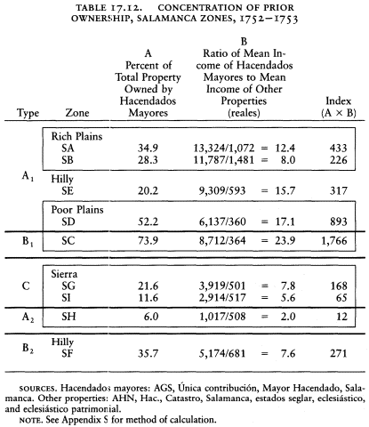
tics. It can be looked on as the area of a rectangle. The vertical side is the percentage of property in the zone owned by the hacendados mayores, and the base is the ratio of the mean income of the properties of the hacendados mayores to the mean income of the other properties (Table 17.12).

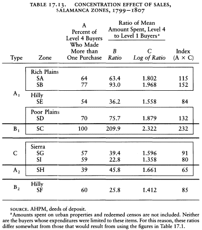
The index of the effect of sales on concentration of landholding is a similar rectangle derived from the sales records. The base of the rectangle also represents a comparison of large to small properties, in this case the ratio of the mean amount spent by the buyers in Level 4 (the largest buyers) to that of the buyers in Level 1 (the smallest buyers). Rather than use the simple ratios, which run from 23 : 1 to 210 : 1, I sub-

stituted their logarithms. The reason is that the range is very high, the largest reading being over nine times the smallest. The other statistic in this index, to be described next, has a range of only 2.6. Multiplying them together would give an excessive weight to the first. The logarithm reduces the range to 1.7, less than that of the other statistic but not so dissimilar.

The vertical side of the rectangle is the percentage of buyers in Level 4 who bought more than one property. At first sight this figure may not seem directly comparable to the percentage of land owned by hacendados mayores used for the earlier index. It was chosen because this index was intended as a measure of change due to the sales, not of the already existing concentration of the lands being sold. Properties being farmed as single units were not ordinarily divided before their sale. Therefore the lowest concentration effect (the greatest increase in the number of landowners through the sales) would result if each property went to a different buyer. The percentage of buyers who bought more than one property is thus a measure of how much concentration was effected above this minimum. It is proper to use only Level 4 buyers in each zone because, smallest in number (they ranged from 3 to 12 percent of all buyers), they had the greatest effect on the pattern of landholding: by definition they accounted for 50 percent of the purchases. The index and its components are given in Table 17.13. (One should stress that even though this index measures the extent to which the sales created new large holdings in the hands of laymen, it is not a measure of the absolute change in concentration. Some religious endowments consisted of various properties that were sold off separately, thus tending to decrease the existing concentration of ownership. The absolute change was the difference between these two contrary effects, which I have not attempted to calculate.)

When the two indexes or sets of rectangles, one of the prior concentration of landowning and the other of the effect of sales on concentration, are compared, they give a high coefficient of correlation, r = .89. Statistically this means that the correlation could have occurred by chance less than once in a hundred cases (it is significant at the 1-percent level). Although the indexes are the products of circuitous calculations, they offer strong support for the validity of the proposition.

Figure 17.1 graphs the result, the regression line of the effect of the sales on the prior concentration. The resulting pattern supports both the division of the zones into types of participation in the market and into geographic regions. Type A₁ zones (SA, SB, SD, SE) fall in the middle of

the pattern, with Type B₁ (SC) far out on its own and Type C (SG, SI) together at the other extreme. Zones in the different geographic regions are even more closely associated, poor plains zones (SC, SD) with high concentration, sierra zones (SG, SH, SI) with low concentration, and zones in the other two geographic regions are also proximate to each other.^[26]

[26] The statistical strength of the correlation depends greatly on the outlier SC. Without it, the correlation coefficient drops to 0.59, and consequently the correlation line swings clockwise. The pattern loses its statistical strength, being valid only at between the 10-percent and 20-percent level. What weakens the correlation is the deviance of Zone SB, which shows a much higher effect of concentration from the sales than the regression would predict.

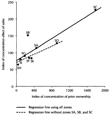
Figure 17.1.
Salamanca Province, Regression of Concentration
Effect of Sales on Concentration of Prior Ownership