Multiperiodic Systems

Since Michelson's measurements of 1891, the hydrogen spectrum was known to exhibit a fine structure: that is to say, most of its spectral lines could be resolved into narrow multiplets. Considering how small it was, this structure could hardly be held against Bohr's theory of 1913. On the contrary, in 1915 Bohr looked for an explanation based on the relativistic correction of the electron mass on a circular orbit of his model. Sommerfeld also tried to explain the fine structure within Bohr's theory, but without relativity. He originally believed that a new quantum condition, when added to Bohr's, would produce the observed splitting.^[24]

In the case of circular orbits the quantum rule (2), , could be rewritten in terms of the polar angle and the conjugate momentum

[24] Bohr 1915a, 334-335; Sommerfeld 1915b. On the empirical discovery of the fine structure see Jammer 1966, 91.

(the angular momentum) as

a form earlier given by Bohr himself.^[25] Sommerfeld, unlike Bohr, applied the latter to elliptic motions, together with the extra quantum rule:

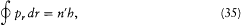
which was to Bohr's rule what the canonical pair (r , P_r ) was to (q , Pq ). The resulting expression for the energy,

was quite disappointing, since it provided nothing but a relabeling of Bohr's terms.

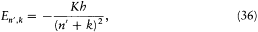
In 1916 Sommerfeld combined his idea with Bohr's appeal to relativity. In this case the motion is no longer strictly periodic: a slow rotation of the main axis around the center of force is superposed upon the Kepler motion; and the energy of the precessing ellipses, quantized according to the above rules, becomes

with x = 2pe² /hc (a derivation of these results will be given after the introduction of the Hamilton-Jacobi method). Since , a good approximation of this formula is

with n = n ' + k . The second term seemed to provide the expected splitting. A quantitative agreement was reached with later experiments, after Bohr and Kramers had derived the necessary selection rules and intensities.^[26]

A few months after the publication of Sommerfeld's results, Schwarzschild and Epstein justified and widely generalized the new quantum rules in two fundamental papers on the Stark effect of the hydrogen atom. They used analytical methods from celestial mechanics to quantize not only the hydrogen atom in an electric field but any multiperiodic system.^[27] Since

[25] For instance in Bohr 1913, 24-25, and Bohr [1916], [451].

[26] Sommerfeld 1915c, 1916a. See Nisio 1973. For the difficulties of an empirical confirmation of Sommerfeld's formula see Kragh 1985.

[27] Schwarzschild 1916; Epstein 1916a, 1916b. See Jammer 1966, 103-104.

these methods played an essential role in the formulation and exploitation of the correspondence principle, I will now present them in some detail. For the sake of clarity I will rely principally on a purified version to be found in the appendices of Sommerfeld's Atombau , with some improvements borrowed from Bohr and Kramers.^[28] The reader already familiar with Hamiltonian mechanics and action-angle variables need read only the paragraph on quantum rules (pp. 110-111) and that on Bohr's golden rule (pp. 115-116).

The Hamilton Jacobi Equation

Consider a mechanical system with the configuration q = (q₁ , . . . q_i , . . . q_s ), the Lagrangian function L (q, q^[*] , t ), and the action integral

For fixed values of q (t ₀ ) and q (t₁ ), the motion between t₀ and t₁ is given by Hamilton's principle dS = 0, which is fulfilled if and only if Lagrange's equations

are satisfied. Alternatively, one may use a Legendre transformation of L ,

This gives the Hamiltonian function H (q, p, t ) and the canonical equations of motion:

H represents the energy of the system; if L does not explicitly depend on time, H is a constant of the motion.

For a fixed value of q (t ₀ ), to a given value of q ₁ and t₁ corresponds (in general) one and only one motion for which q (t₁ ) = q₁ ; the corresponding value of S is noted S (q₁ , t₁ ). An explicit expression of the differential of this function results from the following reasoning. We first consider t₁ to be fixed and q₁ to vary by d q₁ , and denote by d q(t ) the corresponding

[28] Sommerfeld 1919, appendices; Bohr 1918a, par. 3: "Conditionally periodic systems," 16-36; Kramers 1919, 289-294. Burgers 1917 and Born 1925 gave the most general and extensive treatment of the quantization of multiperiodic systems. In this context the most useful treatise of classical mechanics is Goldstein 1956.

variation of the motion q (t ) between t₀ and t₁ . The resulting variation of S is

The second term vanishes by virtue of the Lagrange equations; the first gives d S = p₁ ·d q₁ , since dq ₀ = 0. Consequently,

We now consider a simultaneous variation of t₁ and q ₁ , but along a given motion. Using (39), the resulting variation of S reads:

Using (44), the same variation reads:

Consequently, we have

Finally, combining (44) and (46) and omitting the index 1, we get

We now suppose the system to be conservative (i.e., L does not depend explicitly on t). Since H takes a constant value E during a given motion, one may advantageously introduce the Legendre transformation

through which t is eliminated and E and q become the natural variables:

As results from the latter differential expression, the function S ' obeys the so-called Hamilton-Jacobi partial differential equation:

Suppose that the general integral of the above equation has been found under the form S '(q, a , E), where a =(a₁ , . . .a_i . . . .a _s-1 ) are integration constants (I have omitted a trivial additive constant in S '). Then taking

the derivative of the Hamilton-Jacobi equation with respect to x_i gives

Consequently, the derivative is a constant of the motion. The s — 1 equations

determine a trajectory in q -space, and the equation

the so-called equation of time, specifies the motion along this trajectory. Thanks to this remarkable theorem of Jacobi, the complete solution of the mechanical problem results from simple differentiations, once the general integral of the Hamilton-Jacobi equation is known.

The practical importance of this theorem comes from the fact that most solvable mechanical problems fall into a category to which Jacobi's method is well adapted: namely, one for which the Hamilton-Jacobi equation is "separable," meaning that for a proper coordinate choice it can be split into s independent equations of the type

with

I will now discuss two simple examples of such problems, and some important properties of the resulting motions.

Two Examples

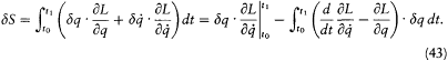
First consider a nonrelativistic system with only one degree of freedom and with the Lagrangian . The Hamilton-Jacobi equation is trivially separated as

which gives

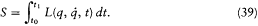
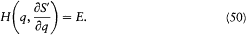
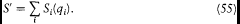
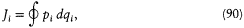
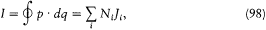
Figure 10.
Form of the available kinetic energy leading to periodic motions.

The equation of time (53) then gives

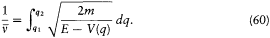
If we limit ourselves to motions capable of corresponding to stationary states, we have to exclude cases for which q can reach infinity or can converge toward a fixed point. This supposes the existence of an interval [q₁ , q₂ ] in which E — V (q ) is positive and at the limits of which it vanishes, as in figure 10, and for which the integral

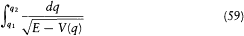
has a finite value. Then q is a monotonous function of time until it reaches either of the extremities of the above interval; at such a point the momentum p = dS'/dq vanishes, and q reverses its motion until it reaches the other extremity with zero velocity, and so forth. The resulting motion is periodic with the period

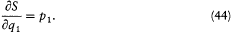
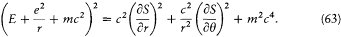
Our second example will be that of relativistic Kepler motion. In any relativistic motion the kinetic energy T is related to the (rest) mass m and to the momentum p by

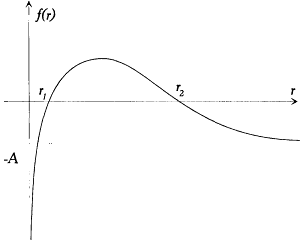
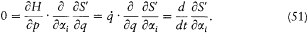
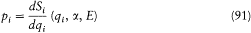
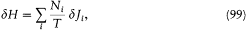
Figure 11.
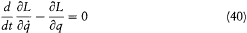
Form of the radial kinetic energy in the Kepler problem.

This implies, for the (binding) energy E = T — e² /r in a Coulomb potential, the equation

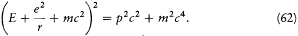
Therefore, the Hamilton-Jacobi equation in polar coordinates (r , q ) in the plane of the trajectory reads:^[29]

This equation is separable according to

with

and

wherein f (r ) = - A + 2B/r - C/r² ,

[29] For the sake of brevity I assume the planarity of trajectories in central potentials to be already known.

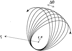
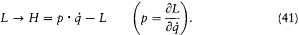
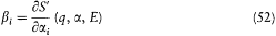
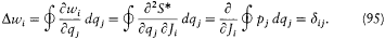
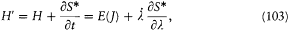
Figure 12.
The relativistic Kepler motion.

For bound motions the energy E must be negative, which implies A > 0; for quantized motions, as will appear later, , which implies C > 0. Consequently the function f (r ) varies as indicated in figure 11.

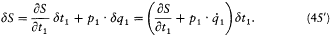
Without recourse to Jacobi's theorem, the general aspect of the motion may be determined by the following simple consideration.

The component P_r of the momentum has the form

where m is the "relativistically increased mass," and it is related to the action S_r by P_r = dS _r /dr . Combined with (66), this implies the differential equation

for the time variation of r . By analogy with the case of the one-dimensional motion treated in the previous example, r must be a periodic function oscillating between the limits r₁ and r₂ of the positive section of f (r ).

The constant Pq = dSq /d q represents the conjugate momentum of q , that is to say, the angular momentum, and is therefore given by

From this equation it results that is a periodic function of time, with the same frequency as the function r(t ). Consequently, after each return of r to its maximal value, the electron describes a portion of trajectory that is simply obtained by a global rotation of the previous portion. The resulting trajectory has the "rosette" shape given in figure 12.

Furthermore, if Dq is the variation of 0 during a period of r (t ) (which is called the advance of the perihelium), the angle

is a periodic function of time with the same period (note that q modulo 2p is not a periodic function). In the complex plane of the trajectory the position of the electron is therefore

the Fourier spectrum of which has only two fundamental frequencies, and

with the harmonics , wherein r is a positive integer. The motion is said to be biperiodic.

Quantum Rules

The following generalization of the above results holds for any separable Hamiltonian system: For coordinates q that allow separation of the Hamilton-Jacobi equation, and for any motion in which none of these coordinates tends toward a fixed point (including infinity), each of the canonical couples (q_i (t ), p_i (t )) repeatedly describes in the course of time a closed trajectory in the (q_i , p _i )-plane, provided that different values of q_i leading to the same configuration of the system are identified (for example, q and q + 2p , if q is an angle). Then, even though the variation in time of these couples is in general not periodic, the motion is multiperiodic: that is to say, the configuration of the system may be expressed in terms of s (or less) periodic functions of time (where s is the number of degrees of freedom), as will be proved after the introduction of the action-angle variables.

For such multiperiodic motions a natural generalization of Bohr's quantum rule lies at hand. As we have seen, the rule (15) for a strictly periodic motion reads (using (20))

Since, in the separated multiperiodic case, p_i = dS _i /dq_i is a function of q_i only, it seems natural to split this rule into s different rules

where the integrations are performed over the closed trajectories referred to in the above discussion of separable systems. In general, these conditions completely determine the energy of the system, since their number is equal to the number of parameters in the action function S '. It remains to prove that the resulting energy spectrum does not depend on the choice of the separating coordinates. This will be done later, after the introduction of the action-angle variables.

Quantization of the Relativistic Kepler Motion

In this case the separating coordinates are the azimuth q and the radius r . Accordingly, there are two quantum conditions. The azimuthal one reads

which expresses the quantization of angular momentum in terms of the "azimuthal quantum number" k . The radial condition reads

or, with the notation introduced in (67),

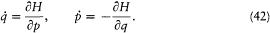
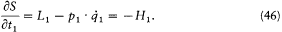
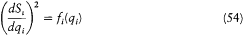
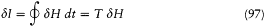
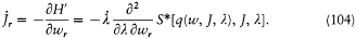
The latter integral is easily computed through the method of residues. In the complex plane the radical has a "cut" along the real segment [r₁ , r₂ ] and two poles, at z = 0 and . The integral J_r is identical with the integral on the loop represented in figure 13, if only the square root is

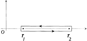
Figure 13.
The slit in the complex plane of the function 

determined to be positive under the cut and negative above it. If this loop is considered to enclose the region outside the small rectangle, Cauchy's theorem gives

where

and is the residue of for u = 0, that is,

The resulting expression for J _r is

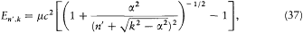
Using the expressions (67) of A, B, C in terms of E and pq , the two quantum rules imply the energy formula (37):

with x = 2p e² /hc for the "fine structure constant." This is, as Sommerfeld put it himself, "the royal road" to the Sommerfeld formula. Needless to say, his first derivation was more hesitating.^[30]

Canonical Transformations

A little before his premature death, Schwarzschild found the method best suited to the determination of stationary states, namely, the introduction of the so-called action-angle variables. Unlike common users of analytical mechanics, astronomers like him sometimes favored this technique, for it provided direct access to the periods of celestial motions. The passage from the original canonical variables to the action-angle variables is a particular case of a more general type of transformation preserving the Hamiltonian structure of the equations of motion. I will first recall some general definitions and results about these transformations.

Since q and p play (anti)symmetrical roles in the equations of motion

[30] Sommerfeld 1919, 327-357, 520-522.

deriving from the Hamiltonian H (q, p, t ), a natural question is: What is the most general transformation from (q, p, t ) to (Q, P, t ) for which there exists a new Hamiltonian K (Q, P, t ) such that

holds? The answer lies in the following theorem.

There exists a function K if and only if the transformation is the result of a combination of the three following types of transformation. The first type simply involves re-scaling

and leads to K = Dm H. The second type involves a permutation

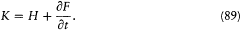
and leads to K = -H . The third type consists of any transformation for which there exists a "generating function" F (q, P, t ) such that p and Q considered as functions of q and P are given by

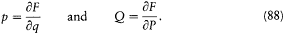
The new Hamiltonian is then given by

Combinations that do not involve a re-scaling are called canonical transformations . For an elementary proof of this theorem I refer the reader to Goldstein's textbook.^[31]

Action-Angle Variables

We now return to a conservative separable system. In a coordinate system for which the Hamilton-Jacobi equation and the action S ' are separated, the action variables are defined as

[31] Goldstein 1956. The type of generating function defined here is not the one most commonly found m textbooks; but it is the most useful, since it includes transformations in the neighborhood of the identity.

where the integrations are performed over the cycles earlier introduced in the (q_i , p_i )-planes. Through the relations

the J 's are in general in a one-to-one correspondence with the parameters x . and E and can therefore be taken as new parameters of the action, according to

As results from , the function S ^* generates a canonical transformation from (q, p ) to (w, j ), with

for the "angle variables."

Since S^* does not explicitly depend on time, the new Hamiltonian is simply the old one expressed in terms of the new coordinates, or E (J ) (the energy of a given motion is completely determined by the action variables only). The new Hamiltonian equations are

The second equation implies a linear variation in time of every angle variable.

The angle variables have another remarkable property. For a given choice of J , the partial variation D w_i of w_i during a "full variation" of the coordinate q_j (i.e., a variation for which the canonical couple (q_j , p _j ) completes a cycle) is

Consequently, the configuration of the system is a periodic function of every w_i with period unity. This is of course why the w 's are called angle variables, even though they generally are not angles in the geometric sense (as the reader will easily verify in the case of the relativistic Kepler motion). Furthermore, for a given motion the configuration is a multiperiodic function of time with frequencies

since, according to (94), the angle variables are linear functions of time with the rate .

Bohr's Golden Rule

As can easily be proved, a system performing a multiperiodic motion returns as close as one wishes to its initial configuration after a sufficiently long time T . This is why a multiperiodic system is also called "condition-ally periodic." Consider a nearly closed motion during the time T and a neighboring motion of the same system. The relation (23) proved earlier for a strictly periodic system gives approximately

The integral I is related to the J 's by

where N , is the number of "cycles" of the couple (q_i , P ,) during the time T . Therefore, relation (97) may be rewritten as

where T/N_i is the so-called "average period" of the coordinate q_i (the variation of which is not periodical in general, as I repeatedly mentioned). In the case where the two neighboring motions are described in the same set of separating coordinates, another expression of D H is obtained by taking the differential of the function E (J ) according to (96),

Comparison with (99) gives and thereby a more intuitive interpretation of the frequency as the average number of cycles of the coordinate q_i in a unit of time.

We now assume that the two neighboring motions are given in two different (but infinitely close) systems of separating coordinates. If, in spite of this change of coordinates, the corresponding J 's are given the same numerical values, the energy remains unchanged according to (99). Consequently, the energy spectrum obtained from the condition J = nh does not depend on the choice of the separating variables, as long as all possible choices are connected continuously. This very elegant proof of the unambiguous character of the Bohr-Sommerfeld rules is due to Bohr.^[32]

[32] Bohr 1918a, 10-12, 22-23.

In the so-called nondegenerate case, for which the frequencies are incommensurable, the arbitrariness in the choice of separating coordinates is limited; only transformations mixing each pair (q_i , p_i ) can be allowed, and the choice of the set of action variables is unique, as Schwarzschild proved. If there are, instead, r (independent) relations

with integral coefficients relating these frequencies, the following transformation is possible. First, the w 's can always be permuted in such a way that the s - r last ones have incommensurable frequencies. Then the function

generates from (w, J ) new action-angle variables (w', J ') such that, for is a constant of any motion and does not appear in the energy expression E (J '); for , is identical with w_i . Consequently, the number of independent quantum conditions is always equal. to the degree of periodicity of the system (that is, the number of independent frequencies). To summarize, greatly benefiting the Bohr-Sommerfeld theory, the introduction of action-angle variables for separable Hamiltonian systems made it easy to derive several important properties: the multiperiodicity of all motions that do not converge toward a fixed point, the unambiguous character of the quantum rules, the degree of multiplicity of the resulting energy spectrum, and the relation (100),

which I will call "Bohr's golden rule" because it subsequently played a fundamental role in the formulation of the correspondence principle. Finally, as J. M. Burgers could show in his important dissertation (1918), action-angle variables were best suited to verify that quantum rules—or action variables—were adiabatically invariant, as required in Bohr's notion of stationary state. The following is a sketch of Burgers's reasoning, which can be omitted at first reading.^[33]

Adiabatic Invariance of the Action Variables

Suppose that the Hamiltonian of the system contains a parameter D and that the system is separable and multiperiodic for every value of D . Then

[33] Burgers 1917, 1918.

there exists a generating function S^* (q, J, l ), defined as in (92), for new canonical variables (w, J ) depending on the parameter l Now assume that l is a function of time with zero value for , a very slow and smooth (in a sense to be later specified) increase for and the constant value for . Before and after the variation of ). the canonical variables generated by S^* are action-angle variables. But during the variation of l , their evolution is ruled by the new Hamiltonian (given by (89))

1

and the J 's are no longer constants, as implied by the canonical equation

To first order in , q(w, J,l ) and S^* may be calculated as if l were constant. In this approximation S^* increases by J_r when w_r increases by one unit, since for a cycle of the coordinate q_r

Consequently, S^* - w·J is a periodic function of each w_r with period one. The same is true for the derivative

which therefore admits the Fourier development

The resulting Fourier series for the second derivative occurring in (104) is

After substitution of , the time average of this expression over a long time (much longer than any period of the motion) is zero, unless there exists a sequence t of integers for which without t _r being zero. Roughly, this singular case does not occur as long as we limit ourselves to transformations for which the degree of degeneracy of the system does not change.^[34]

[34] Unfortunately, this condition is never rigorously met, as realized by Burgers himself. Complete proofs were given as late as 1924 by Dirac and Laue (see part C, p. 306).

The total variation of J_r during the adiabatic transformation is given by

If we take the variation of to be negligible during the periods of the motion, in the latter integral f_r may be replaced by its average value over a large number of periods, which we just proved to be zero. This seals the proof of the invariance of the action variables J for any adiabatic transformation that does not alter the degree of degeneracy of the system.^[35]

The extension of Bohr's theory to multiperiodic systems raised a general wave of enthusiasm. As Sommerfeld and Born put it, the Hamiltonian formulation of classical mechanics almost seemed to have been created for the sake of quantum theory. The action variables of celestial mechanics permitted a strikingly simple expression of the quantum rules, and the theory of complex integration, a no less beautiful mathematical tool, appeared to be very well suited to the remaining calculations of the energy spectrum.^[36]

In the following years, theoreticians of the Munich and Göttingen schools generally concentrated their attention on systematically carrying out the Bohr-Sommerfeld quantization procedure; they tended to neglect all aspects of quantum phenomena that did not fit into this well-defined mathematical framework (for instance, the intensities of spectral lines). As we shall presently see, Bohr reacted in a quite different way: in spite of his admiration for the concrete achievements of these schools, he emphasized the still provisional and incomplete character of the newly extended quantum theory; he insisted on a careful analysis of the degree of compatibility between the various physical concepts involved, and he concentrated his attention precisely on the questions to which the mathematical art of quantization by itself gave no answer.