Examples of BDSN Seismograms
The dynamic-range and bandwidth capabilities of BDSN recordings are illustrated in figure 3 where a small (ML = 1.7) local earthquake was recorded simultaneously with the surface waves from a large (Ms = 6.8) teleseism. The events have dominant periods of 0.37 s and 23 s respectively and are thus readily separable by convolution or filtering.
Figure 4 shows the spectrum of a local earthquake (ML = 3.1, D = 12 km) recorded by the MHC broadband digital seismograph. The inset waveform is the transverse-component (clockwise up) displacement time history (10-s record). Note the presence of the near-field ramp commonly observed on broadband displacement seismograms for D less than 20 km. The upper curve is the spectrum of the inset seismogram, and the lower curve is the spectrum of a 10-s noise sample immediately preceding the event. The signal-to-noise ratio is approximately 50 dB (a factor of about 300) in the 1–2-Hz frequency band. The steep slope at 5 Hz is due to the 10-pole low-pass anti-aliasing filter.
Calculation from the asymptotic low-frequency spectrum level of 6,500 nanometer-seconds yields a seismic moment of 1.7 × 10²¹ dyne-cm. This earthquake is a factor of five below full scale on the 16-bit telemetry system in the spectral domain at 1–2 Hz. It follows that the largest events that can be recorded on scale at 18 km are ML

A strong regional earthquake, M L = 5.2, recorded at MHC is shown in figure 5. This earthquake occurred adjacent to the Parkfield segment of the San Andreas fault and serves to indicate the seismic ground-motion ampli-
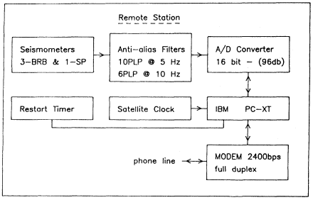
Figure 2a
Remote-station block diagrams showing principal hardware components.
The A/D converter and the restart timer plug into the PC system bus,
while the clock and modem connect to asynchronous serial ports.
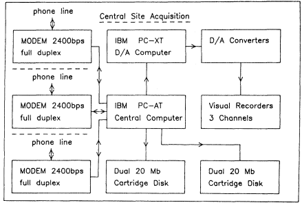
Figure 2b
Central-station block diagram showing principal hardware components.
The D/A converters and the cartridge disk drives plug into the
PC system bus, while the modems attach to asynchronous serial
ports. All components are available commercially.
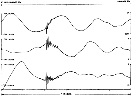
Figure 3
Bandwidth and dynamic range illustrated by a ML = 1.7 local earthquake
(D = 22 km) superimposed on the surface waves from a Ms = 6.8 teleseism
(D = 58°). Full scale (700 counts) corresponds to 18.75 micrometers/second
ground velocity.
tude expected in a characteristic Parkfield earthquake (Ellsworth et al., 1987). The MHC broadband system should remain on scale for earthquakes up to M L = 5.8 in the Parkfield area.
Figure 6 shows the records from a large teleseism (Ms = 7.1 ) that occurred in the Santa Cruz Islands on July 6, 1987. This was the first major earthquake recorded by the Berkeley broadband network since the new BDSN digital equipment has been in operation at BKS and MHC. The MHC, ORV, and SAO traces are from Streckeisen STS-1 instruments (broadband velocity output), the WDC (vertical component only) and BKS traces are from Sprengnether S-5100 series instruments, and the CMB traces are from Teledyne SL 200 and SL 210 instruments. All traces are derived from velocity outputs except for BKS which has displacement outputs. Note the similarity in the body-wave traces and the differences in the surface wave envelopes.