One—
The Development of Global Earthquake Recording

R. D. Adams

The Purpose of Seismological Recording

Seismological observatories and networks have to provide the raw information on which seismology is based. The obvious aim of seismological recording is the location of earthquakes, but there is a duality in observational seismology between the determinations of earthquake positions and of earth structure, for to find each, we need the other. Jeffreys and Bullen (1935) were faced with this problem in the determination of their travel-time tables and refined both tables and locations together, and this process of refinement continues.

Earthquake location in time and space is needed for a variety of reasons, for example, seismic hazard assessments for the engineering and insurance industries and to help local authorities in civil protection planning and preparedness endeavors. The position of earthquakes is also of scientific importance in delineating the Earth's tectonic activity, to show the broad pattern of its major zones and also to give details of occurrence in particular areas for scientific understanding of earthquake processes. An obvious example is the early mapping of the midoceanic ridges by earthquake locations before their bathymetric continuity was established.

Once the positions of earthquakes are known we can use the energy recorded from them to establish the properties of earth structure, including near-surface inhomogeneities and deeper structure and discontinuities, as in recent detailed studies of the core-mantle boundary (Morelli and Dziewonski, 1987). As well as velocity structure, we find the attenuative properties of the Earth from decay of body waves, surface waves, and free oscillations.

The final type of information available from seismograms helps reveal the mechanism of the earthquake source itself. This type of information has obvious scientific interest and often has a practical bearing on questions of

seismic hazard assessment. Source mechanism studies have developed from early work that depended only on the directions of the first motion of P-waves to a modeling of P-wave shape and to analysis of the entire waveform to give additional parameters such as the rupture-time history. It is satisfying that such determinations of source parameters are now closely linked, through techniques such as centroid-moment tensor solutions, with earthquake location, giving another example of a unified approach to seismological problems.

Our seismological observatories must provide the raw information necessary to solve these problems. Little, however, can be achieved by one station alone. Cooperation is the key to success, cooperation among countries, among agencies, and among individual stations to form networks on national, regional, and global scales.

Historical Development of Earthquake Location

Pre-Instrumental

In considering the development of earthquake location, we must not neglect the contributions made by noninstrumental seismology. The reporting of earthquake effects is still a major part of observational seismology and a useful adjunct to instrumental recording, but until a century ago it was the only method of studying earthquakes and their distribution. One of the earliest attempts at a global earthquake plot was a catalog produced by the Irish scientist Robert Mallet (1858). This was based entirely on felt reports, thus missing the details of major seismic features of the oceanic ridges, and showed a combination of population and earthquake distributions. Nevertheless, it was a creditable first approximation to a world seismicity map.

Among others prominent in early studies of global seismicity was the French observer Montessus de Ballore (1896), who published a paper with the impressive title "Seismic Phenomena in the British Empire" and realized the need to distinguish between places where earthquakes were reported felt and actual centers of vibration. He also produced early hazard maps, including one for the British Isles (fig. 1).

Good pre-instrumental information may still be subjected to analysis techniques developed later. An example is Eiby's (1980) analysis from the diaries of a clergyman in Wellington who meticulously noted the time and characteristics of aftershocks of the large 1848 earthquake in the north of the South Island of New Zealand. This provided good estimates of the relative numbers of large and small earthquakes (magnitude-frequency parameter b ) and rate of decrease with time of the numbers of aftershocks (decay parameter p ).

Figure 1
Hazard map of Britain (Montessus de Ballore, 1896). Distances
given in kilometers are an arbitrary measure of seismicity inversely
related to the number of earthquakes in a given region.

Early Instrumental Seismology on a Global Scale

World networks of seismographs, such as the Worldwide Standardized Seismographic Network (WWSSN), the Global Digital Seismographic Network (GDSN), and the Incorporated Research Institutions for Seismology (IRIS), are not new. Early outstations were set up by European countries, such as the German station at Apia in Samoa in 1902, but the first serious attempt at global coverage was the network of the British Association for the Advancement of Science (BAAS) established by Prof. John Milne on his return to Britain from Japan in the late 1890s. The Milne network at its peak had about ten stations in the British Isles and nearly thirty elsewhere throughout the world. The network comprised instruments of standard manufacture from which Milne collected readings at his home in the Isle of Wight in the first systematic analysis of global seismicity. From this enterprise, whose results were published as the Shide Circulars of the BAAS, there developed the International Seismological Summary (ISS) and, later, the International Seismological Centre (ISC). Under Milne, for the first time the true pattern of instrumentally determined global seismicity began to emerge, as shown in his earthquake map for 1899, which also shows the distribution of Milne seismographs (fig. 2; Milne, 1900).

We must remember that the knowledge of earth structure at that time was very elementary, and the instruments low in magnification (about 12), long in period (about 12 s natural period), and undamped, with surface waves as the main recordings. The general accuracy of location was surprisingly good, but naturally mistakes are apparent in the light of modern knowledge. One great strength of the network was its uniformity, which has helped in a recent reevaluation of Milne's locations of early events in West Africa (Ambraseys and Adams, 1986). Irrespective of details, it was often possible to establish by a similarity of reporting that certain stations were nearly equidistant from a given earthquake. We found that consistent locations could be found by using the reported time of the maximum oscillation, M , assuming it to be an Airey phase of velocity 2.8 to 3.0 km/s. In this way we could confirm the location of many early events, but some we found to be grossly misplaced. An example is the event of May 21, 1910, originally placed in Niger in Central Africa but found by us to be in Turkey, where there was confirmatory felt information (fig. 3).

Damped instruments of greater sensitivity were developed after about 1910, and fuller details of P and S phases were recorded but at the expense of uniformity of recording. By 1930 the number of recording stations had grown, and a map (fig. 4) compiled by Miss Bellamy (1936) of ISS shows well the main features of global seismicity, but with the details blurred by scatter. The stations at that time are shown in figure 5.

The number of stations grew steadily, and by 1951 about 600 were listed with their direction cosines in an ISS publication. The distribution of sta-

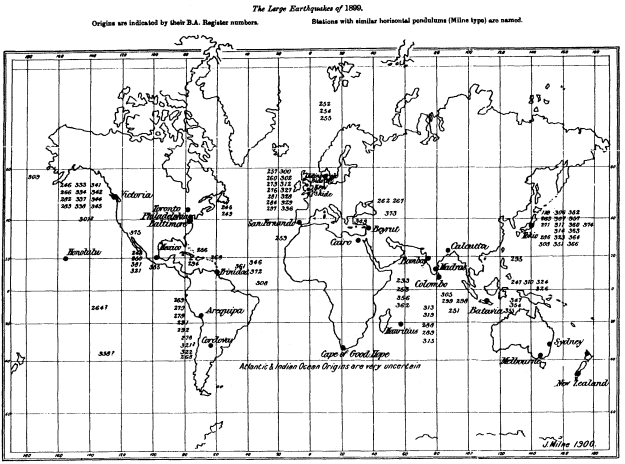
Figure 2
Global earthquakes and seismograph stations in 1899 (Milne, 1900). Epicenters
are approximately indicated by numbers that refer to events in Milne's catalog.

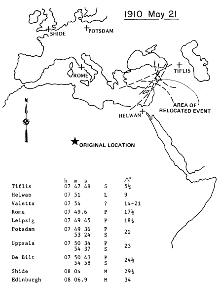
Figure 3
Relocation to Turkey of an event originally placed in Niger (Ambraseys
and Adams, 1986). Arrival times are given for stations with reinterpretation
of phases and derived distances in degrees.

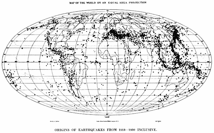
Figure 4
Global earthquakes 1913–1930, showing scatter of features now better defined (Bellamy, 1936).

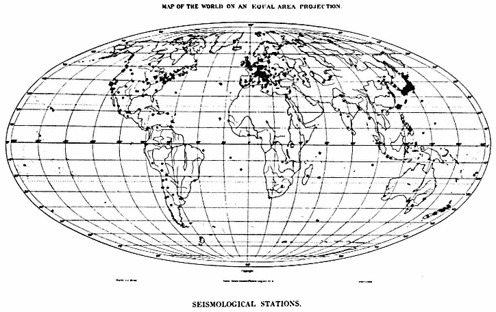
Figure 5
Seismograph stations in 1936 (Bellamy, 1936).

tions, however, remained very uneven, with strong concentrations in North America and particularly in Europe. At the time the New Zealand station Roxburgh was installed in 1957, at latitude about 45°S, it was the most southerly regularly operated station in the world, still leaving the southernmost thirty percent of the world's surface with no station. The advent of the International Geophysical Year, and the installation of about 120 WWSSN stations in the late 1950s and early 1960s, changed the picture enormously; since then the coverage of recording stations has significantly improved.

Felt Reporting

The contribution to observatory seismology of felt information, even in present times, must not be underestimated. Properly documented felt reports can add valuable information, and in some parts of the world they still provide the most accurate locations. Felt reports of a small earthquake often give a more reliable location than can be determined from readings at a few stations, and a well-determined felt pattern for a large event will define the center of energy release, which may be closer to the centroid-moment tensor solution than to the less significant point of initation of rupture that is given by the instrumental hypocenter. Ambraseys and his co-workers (for example, Ambraseys and Adams, 1986) have developed formulae for estimating surface wave magnitude, M_s from isoseismal radii. These estimates have been shown to agree well with instrumentally determined values.

Global Earthquake Location at the Present Time

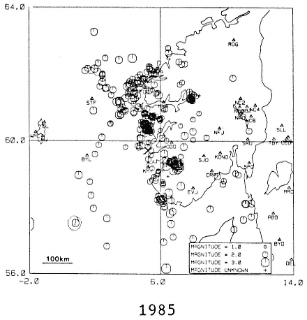
The precision of earthquake location continues to improve. A recent example from the North Sea (Engell-Sørensen and Havskov, 1987) shows a much clearer pattern for 1985, when an improved station network was operating, compared with earlier years (fig. 6). On a global scale many small-scale tectonic features are now apparent in careful plotting of ISC data. Examples of these have recently been produced by Young et al. (1987) of the Ministry of Defence Seismological Unit in Britain (figs. 7, 8).

Despite these advances, some difficulties remain in global earthquake location, and some improvements could still be made.

In 1985, the period on which ISC is now working, about 1,400 stations reported each month, the largest events being reported by about 700 stations. For accurate location, however, it is the distribution of stations, rather than their number, that is important. More stations in seismically quiet, well-developed countries add little to location accuracy. It is true that a few strategically placed sensitive stations, particularly if they are arrays, can detect all major earthquakes, but give poor accuracy of location. Simple array locations of teleseisms are often many degrees in error and can have

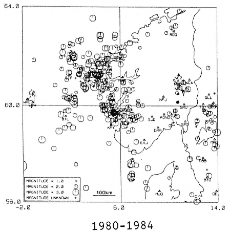
Figure 6a , b
Earthquakes in the North Sea, showing better-defined seismicity for the later
period during which more stations operated (Engell-Sørensen and Havskov, 1987).

compensating errors of up to 600 km in depth and one minute in origin time.

A few currently active stations in remote areas are still of immense value in effective global earthquake coverage. Examples are stations in the Antarctic and those like Raoul Island in the Kermadecs, which is still visited by ships only two or three times a year. Such stations are valuable even if local variations from a spherically symmetric velocity model are ignored.

Let me summarize the present-day status of global earthquake location as seen from ISC. Large major earthquakes are now well controlled in position, including depth, and mechanism. At the other end of the scale, in areas with

close local networks such as California, Japan, and New Zealand, small local earthquakes can be detected and accurately located down to microearthquake levels. Many uncertainties remain, however, for small to moderate events in remote regions, including oceanic areas and sparsely inhabited continents.

The main difficulty in global earthquake location at the ISC is the "association" of individual readings into events. ISC locates about 25,000 events a year, or about one every twenty minutes. Therefore, it is not surprising that considerable ambiguity often arises as to which event a particular arrival belongs. This task is even more difficult at ISC because the analyst has to rely on reported times only, with no additional information on the character of the arrival to help discriminate between phases from teleseisms and local

Figure 7
Detailed seismicity plot of ISC locations (Young et al., 1987).

events. Sometimes the inclusion or exclusion of a particular observation makes two solutions widely separated in position or depth equally plausible.

In addition to uncertainty of station association, detection is still poor in a surprisingly large area of the world. In 1983, for example, ISC found more than 2200 previously undetected new events (about 6 a day) of which 57 (about one a week) had a body-wave magnitudes, m_b , of 5.0 or greater. Most of the new events were found in remote areas around the Pacific, such as the Kermadec Islands, Sunda Arc, and New Guinea, but many also are found in highly active areas such as Turkey and South America, and a surprising number appear in well-developed countries where the national networks cannot locate events by themselves. An example of this is found in Europe, where new events tend to cluster near national boundaries where no one

country has enough information to locate an event, but the combined readings collected at ISC give a satisfactory solution (fig. 9; Adams, 1981). Other new earthquakes have been found in areas previously thought to be aseismic or of very low seismicity, such as Antarctica (Adams and Akoto, 1986).

Another emerging difficulty is analysis that is too automated. In particular, readings of distant events across small, dense networks can be interpreted as local events, either inside or very close to the network, if the records are not carefully scanned for clues of character, for duration, and for later phases. One example occurred on May 23, 1985, when the procedures used at the U.S. National Earthquake Information Center (NEIC) found enough readings from Fijian stations to produce a solution giving a shallow local event, whereas incorporation of readings from more distant stations showed that the earthquake was 500 km deep and nearly 1000 km away (fig. 10). Perhaps the worst recent example is the misinterpretation at the Large Aperature Seismic Array in Montana (LASA) of steeply arriving core phases as P arrivals from the limit of P-wave distance. This results in a spurious "ring of fire" at a distance of about 100° from LASA. In particular, such arrivals from Pacific events form a fictitious zone of activity through Central Africa (fig. 11), which could easily be mistaken for a manifestation of the Cameroon Volcanic Line (Ambraseys and Adams, 1986).

The other great uncertainty in earthquake location that persists is due to the large-scale regional departures in velocity from the accepted models. In particular, the main subduction zones have velocity anomalies of ten percent or more that are ignored in standard processing. For large events located with many teleseismic readings, the errors are minimal, but close stations can exhibit very large residuals. At the other end of the scale, very small events located only by very close stations cannot be greatly mislocated. Intermediate-magnitude events located by a few regional stations can be grossly mislocated, with small residuals arising not from accurate location but from accommodation of inappropriate velocities by the least-squares procedure. An example of this is a 1975 New Zealand earthquake, with a solution from twenty local stations, which by a special study was shown to be mislocated in both position and depth by about 50 km (fig. 12; Adams and Ware, 1977).

Ideally, a complete three-dimensional velocity model of the Earth is needed to ensure good earthquake location. Simple time corrections for stations and sources near areas of velocity anomalies are not enough without considering azimuthal effects. For a first approximation, a "path correction" for each source-receiver pair would give significant improvement.

The reliability of global earthquake location is steadily increasing, but remaining uncertainties are not always appreciated by nonspecialists. Any poorly recorded event in an unusual position should be carefully examined.

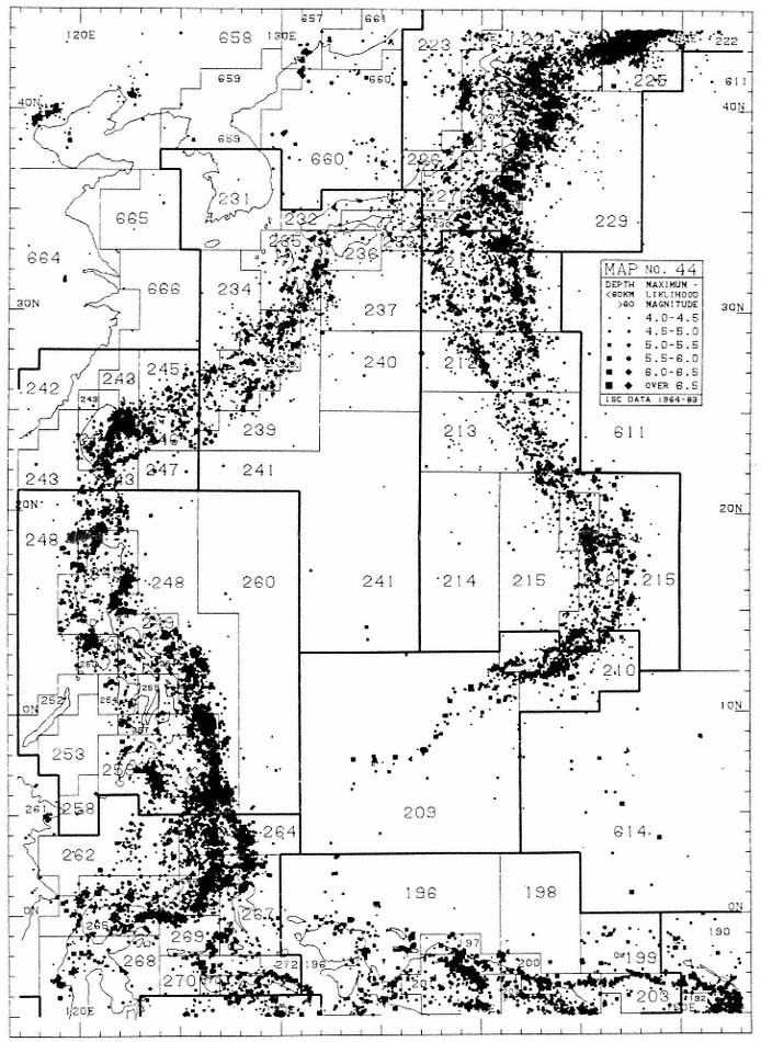
Figure 8
Detailed seismicity plot of ISC locations for the Philippine Sea area (Young et al., 1987).

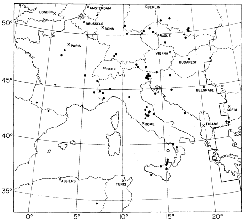
Figure 9
Previously undetected earthquakes in Western Europe found by the
ISC "search" procedure. Note the clustering near international boundaries.
Open symbols represent subcrustal earthquakes (Adams, 1981).

Future Developments

The world network can now adequately locate major earthquakes, and plans of organizations such as IRIS will ensure that detailed studies of their mechanisms can be carried out. It is the smaller events that need closer study, with better velocity models and readings from more and closer stations. The full global seismicity pattern can never be adequately monitored by one hundred or so well-placed sensitive stations. Whereas such a network might detect a large number of events, its accuracy of location would be poor. For example, the locations during a trial experiment in 1984 by stations con-

Figure 10
The ISC computer solution for the earthquake of May 23, 1985. Note the false position found by the U.S. National Earthquake
Information Center because its automatic location procedure misinterpreted readings at stations of a dense local network in Fiji.

tributing to the network sponsored by the Committee on Disarmament, Geneva, were significantly fewer and poorer than those found later by ISC for the same period. The greatest uncertainty in geometric location procedures is still in the determination of depth, and it is here that waveform modeling can make an important contribution.

What developments should be seen by the end of this century? Obviously, there will be an established global network of digital broadband stations, with a dynamic range high enough to record ground noise at the quietest sites but not subject to overload when recording strong motion from major earthquakes. We should also see more close networks in active areas and, in particular, many more stations in remote and oceanic regions, with a great

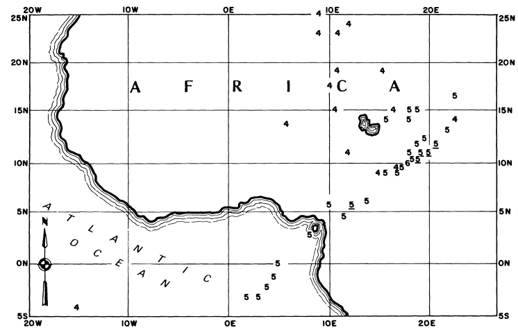
Figure 11
Spurious earthquake locations in Central Africa derived from misinterpretation of core phases on Pacific earthquakes recorded at
the LASA array in Montana. Figures are assigned magnitudes, and underlining implies more than one event at the same location.

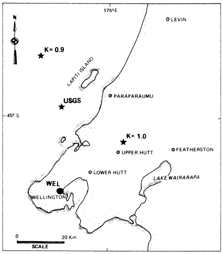
Figure 12
Mislocation of an intermediate-depth New Zealand earthquake. The position indicated
by k  = 1.0 is that found from the local network with a standard velocity model. The
position marked "USGS" is that derived by the U.S. Geological Survey PDE service.
That marked k  = 0.9 is found by special study using a laterally changing velocity
model, and is believed to be closer to the true position (Adams and Ware, 1977).

increase in the number of ocean-bottom seismographs. It has even been suggested that a succession of recording hydrophones be allowed to drift along the major ocean currents. Telemetry by land line, radio, or satellite will bring information for more rapid determination of earthquake parameters, but later, more refined processing will still be needed, as now, with careful monitoring by trained seismologists. The later analysis will include not only refinement of location, but modeling for depth and mechanism.

Observational seismology has come far in the last hundred years. There is every prospect that it will continue to develop and prosper.

Acknowledgments

I thank Dr. P. W. Burton of the British Geological Survey for supplying early seismicity maps, and Mr. J. B. Young of the Ministry of Defence Seismological Unit, Blacknest, for permission to use previously unpublished plots of ISC earthquakes.

References

Adams, R. D. (1981). ISC determinations of previously unreported earthquakes in Europe. In V. Schenk, ed. Proceedings of the 2d International Symposium on the Analysis of Seismicity and on Seismic Hazard, Czechoslovak Academy of Sciences, Prague, 132–139.

Adams, R. D., and A. M. Akoto (1986). Earthquakes in continental Antarctica. In G. L. Johnson and K. Kaminuma, eds., Polar Geophysics. J. Geodynamics 6: 263–270.

Adams, R. D. and D. E. Ware (1977). Sub-crustal earthquakes beneath New Zealand; locations determined with a laterally inhomogeneous velocity model. N. Z. J. Geol. Geophys., 20: 59–83.

Ambraseys, N. N., and R. D. Adams (1986). Seismicity of West Africa. Ann. Geophysicae, 4B; 679–702.

Bellamy, E. F. (1936). Index Catalogue of Epicentres for 1913–1930. County Press, Newport, Isle of Wight. United Kingdom, 36 pp.

Eiby, G. A. (1980). The Marlborough earthquakes of 1848. New Zealand DSIR Bulletin 225, 82 pp.

Engell-Sørensen, L., and J. Havskov (1987). Recent North Sea seismicity studies. Phys. Earth Planet. Inter., 45: 37–44.

International Seismological Summary (1951). The geocentric direction cosines of seismological observatories. County Press, Newport, Isle of Wight, United Kingdom, 18 pp.

Jeffreys, H., and K. E. Bullen (1935). Times of transmission of earthquake waves. Bureau Central Séismologique International, Travaux Scientifiques, Strasbourg, 11.

Mallet, R. (1858). Fourth report upon the facts and theory of earthquake phenomena. Report of 28th meeting of British Association for the Advancement of Science. John Murray, London, 1–136. (Plate XI).

Milne, J. (1900). Fifth Report of the Committee on Seismological Investigations Plate II,. British Association for the Advancement of Science, London.

Montessus de Ballore, F. de. (1896). Seismic phenomena in the British Empire. Q. J. Geol. Soc. Lond., 52: 651–668.

Morelli A., and A. M. Dziewonski (1987). Topography of the core-mantle boundary and lateral homogeneity of the liquid core. Nature, 325: 678–683.

Young, J. R., R. C. Lilwall, and A. Douglas (1987). World seismicity maps suitable for the study of seismic and geographical regionalisation. AWRE Report 07/87. Her Majesty's Stationery Office, London.