FOUR
The Value of Rate Reform in a Competitive Electric Power Market

Richard J. Gilbert and John E. Henly

I. INTRODUCTION

The 1980s signaled a new pattern of competition in the electric power industry. Increased capital costs resulting from newly completed construction projects boosted utility rates at the same time that lower oil and gas prices and procompetitive legislation, led by the Public Utility Regulatory Policies Act, provided alternatives to utility-generated power.

These changes in utility costs and industry structure undermined the economic performance of California's electric rate structures (as well as those of other states). Features of California's rate structure that could be defended on economic efficiency grounds in the late 1970s and the early 1980s were impediments to economic efficiency in the late 1980s and, if not altered, will probably continue to have adverse consequences through the turn of the century.

The features of the current pricing system that are particularly troublesome in this new environment are: (1) the increasing block tariffs faced by residential customers, (2) the application of traditional cost recovery practices to recently completed construction projects, and (3) the subsidization^[1] of residential and agricultural customers by industrial and commercial customers. These features drive electricity prices away from marginal costs. As a result, businesses are driven away from least-cost

[1] There is no universal definition of subsidization. However, in California the markup of price over marginal cost is less for residential and agricultural customers than it is for other customer classes, and in conjunction with class elasticities and rate structures, the effect of this is to decrease economic efficiency as shown in the section on subsidization later in this chapter.

production techniques, and consumption decisions are distorted by prices that are removed from marginal costs.

Regulators and state legislators may, of course, pursue goals other than economic efficiency, but it is important from a policy standpoint to place a price on those goals. In this chapter we attempt to determine this price. We calculate that a failure to respond to recent changes in the utilities' cost structure in an economically efficient way would cost northern California's businesses and consumers approximately $400 million a year (levelized) over the 1987-2003 period. Extrapolating these results to the entire state indicates a cost of approximately 1 billion per year on a levelized basis.

Our results indicate the need for a coordinated approach to utility rate design. If utility revenues are required to cover costs, a change in the allocation of revenue responsibilities across customer classes alone cannot achieve significant efficiency gains without large distributional impacts. Moreover, changes in the pattern of cost recovery over time have limited scope for efficiency gains without large accompanying changes in customer rates. But it is possible to design an efficient rate structure that is distributed more acceptably if changes in customer rates are coupled with changes in the pattern of utility cost recovery over time.

In the next section we discuss qualitatively how changes in cost structure and technology have reduced the economic efficiency of electric rate structures similar to California's. Then we describe our methodology and the dynamic simulation model used to measure the effects of rate structure changes on economic efficiency. We measure the gain in economic efficiency that would result from changing the 1986 rate structure^[2] to marginal-cost pricing for a utility modeled after the Pacific Gas and Electric Company (PG&E), California's largest electric utility. We explore the efficiency effects of specific features of the California rate structure by "improving" them (in terms of economic efficiency) while holding other characteristics of the rate structure constant. We look at alternatives to traditional utility cost recovery practices, assuming uniform rate schedules. Revenue requirements are shifted among industrial, commercial, and residential rate classes using Ramsey and modified Ramsey criteria to determine how the allocation of revenue requirements among customer classes affects economic efficiency when marginal-cost pricing is not possible. Recognizing that political and equity constraints limit rate reform, we conclude the quantitative analysis by discussing a rate structure that achieves more than one-half of the efficiency benefits of marginal-cost pricing while at the same time making some concessions to likely political constraints. Finally, we attempt to place our results in a broader policy perspective in the conclusions.

[2] We use the 1986 rate structure as a base case.

II. THE PROBLEM

Perhaps no economic result is more widely cited by economists than the efficiency of pricing at short-run marginal cost.^[3] Setting prices for mar, ginal consumption at marginal cost forces buyers to weigh the benefits of marginal consumption against its cost consequences. In the electric utility industry short-run marginal cost is best thought of in probabilistic terms. An additional unit of electricity demand imposes several types of expected costs on the electric system and/or other customers. These costs include fuel costs, maintenance costs, operating costs, and shortage costs. The term expected is used because actual costs are not known in advance, even in the very short run. This is most important with regard to shortage costs. Shortage costs occur because the addition of another unit of demand increases the probability of an outage or brownout, events that impose large costs on other customers and also on the utility, but that occur only with small probability.^[4] Although the occurrence of events that cause a shortage (e.g., failures of generating equipment and transmission lines, overloads of equipment, weather damage) cannot be predicted with certainty, the probability of such events creating a shortage can be used to determine expected marginal shortage costs as a function of demand conditions. In this chapter, the term marginal costs should be thought of in this expected-value sense. The efficient price of electricity includes expected marginal shortage costs (Crew and Kleindorfer, 1976; Chao, 1983). Marginal fuel costs and marginal operating costs can also be considered probabilistically, but actual values for these costs can be forecast in the short term with much greater accuracy.

Changes in the cost structure of the electric industry have raised electricity prices well above marginal costs. Figures 4.1 (1980) and 4.2 (1986) illustrate these changes in cost structure based on PG&E data. Although indicative of actual utility cost conditions, the position of these curves is approximate and should not be interpreted as a literal descrip-

[3] There are exceptions, to be sure. Systematic misinformation about the private costs and benefits of marginal consumption, differences between private and social costs or benefits, and inefficient pricing in related markets can all be reasons for the efficient marginal price to differ from marginal private cost. Lee Friedman discusses possible effects of limits on information and information processing abilities in Chapter 2. However, in any scheme where price plays a role in determining the quantities consumed, marginal cost will play an important role in determining the efficient price. Changes in marginal cost will require appropriate changes in price, if efficiency is to be maintained.

[4] Shortage costs can result from bottlenecks in generation, transmission, or distribution and can be thought of as a congestion externality. The portion of these costs borne by utility customers should be reflected in the efficient price of electricity, even though it does not add directly to the utility's revenue requirement. Of course the portion of expected marginal shortage costs that do add to the utility's expected revenue requirement should also be reflected in the efficient price.

tion of the PG&E cost structure. In particular, actual costs depend on hydro conditions, factor prices, and supply contracts.

Average cost in Figures 4.1 and 4.2 is equal to average revenue requirements, the amount that would have to be collected per kilowatt-hour (kWh) to raise enough revenue to cover costs, including a normal return on shareholders' investment. In 1980 average cost is almost constant over a wide range of production around yearly sales of about 60,000 gigawatthours (GWh/year). Marginal fuel costs depend on the rate at which electricity is produced and increase rapidly at production levels greater than 60,000 GWh/year, reflecting the low thermal efficiency and high fuel costs of marginal sources of power used at higher demand levels. Total marginal costs are greater than the marginal fuel costs pictured, because they include items such as marginal maintenance costs, other marginal direct operating costs, the cost of carrying that portion of working capital and fuel inventory that varies with demand, and expected marginal shortage costs. The addition of these other marginal costs raises expected marginal costs above the level of average revenue requirements in the pre-1986 period. Pricing all electricity at expected marginal cost during this period would have brought in more revenue than was needed to cover costs.

Since the 1970s, California and some other utility systems have had an increasing-block-rate structure for residential customers, in which the marginal price increases in steps with use (see Figure 4.3).

In the high marginal-cost and (relatively) low average cost environment that prevailed until 1986, increasing block rates for residential customers^[5] and a subsidy to the residential class from other customers were defensible on economic efficiency grounds, because both of these characteristics of California's electric rate structure moved marginal prices toward marginal costs. With increasing block rates the marginal price of electricity (i.e., the price customers pay for their marginal consumption) will usually be greater than the average price. Thus it is possible in theory to charge a marginal price roughly equal to marginal cost and, as a result, gain efficiency benefits without raising more revenue than is needed to cover costs. We do not claim that this was the state legislature's primary motivation for instituting increasing block rates or that particular rate schedules were designed primarily for their economic efficiency properties. However, during the period that marginal costs exceeded average revenue requirements, increased efficiency was at least a likely by-product of increasing-block-rate structures.

[5] In California increasing block rates have historically gone by the names of "lifeline" and "baseline" and have consisted of two to three tariff blocks, depending on the time period and the utility.

Increasing-block-rate schedules were not used to price electricity for nonresidential customers in California.^[6] Instead, relatively uniform rate schedules were in effect for these classes.^[7] The increasing block rate structure for residential customers shifted part of the burden of covering revenue requirements to the nonresidential customers. With high system marginal costs, the effect of this shift was to move nonresidential prices closer to marginal cost in the pre-1986 period. The combined effect of increasing block residential rates and higher nonresidential rates was to move marginal prices in the direction of marginal costs in the pre-1986 period for all customer classes.

Figure 4.2 illustrates the 1986 cost structure at PG&E. As a result of lower-than-expected demand growth and large capital additions, average revenue requirements per kWh are higher than in 1980 and decline rapidly in the neighborhood of 1986 consumption (about 65,000 GWh). Marginal fuel costs, dominated by lower oil and gas prices and the greater thermal efficiency of plants at the margin of production, are rising only slowly at this output and are far below average revenue requirements. Marginal shortage costs are also much smaller in 1986 than in 1980, reflecting ample reserve margins in 1986.

Increasing block rates for residential customers continued to characterize rate structures in 1986 despite massive changes in the industry's cost structure. In addition, the price/marginal-cost gap has been larger for nonresidential customers, implying a subsidy^[8] to the residential class and higher marginal prices for all consumers. Under the post-1986 cost structure, increasing block rates and high industrial and commercial rates move prices away from marginal cost (which is much lower than the average per-kWh revenue requirement). As a result, in late 1986, electricity prices at California's largest utilities were more than three times marginal fuel costs. Table 4.1 gives the California Energy Commission's (CEC's) estimates of 1987 prices and marginal fuel and marginal shortage costs for each of the three major investor-owned utilities in the state.

The large gap between price and marginal cost is likely to be a long-term phenomenon. Figure 4.4 is a 17-year projection of the relationship between total annual revenue requirements for PG&E and marginal-cost revenues (the latter defined as the revenues collected at the same output

[6] For various reasons, including different impacts on costs of competing firms, block rates may not be an efficient or equitable way of pricing electricity to nonresidential customers. Ordover and Panzar (1980) provide a specific example of adverse efficiency effects under certain circumstances. Because nonresidential customer classes are quite heterogeneous, equity problems also arise with block rates.

[7] Although charges may vary depending on the time of use or according to the proportions of power and energy demanded, price does not vary much as a function of output, holding these other factors constant.

[8] At the time this chapter was being written, the CPUC was considering proposals to reduce the extent of residential subsidization by other customer classes.

level if prices were set at marginal cost), assuming a 3.2% real annual increase in marginal costs and traditional cost recovery for capital expenditures. Marginal costs in Figure 4.4 include marginal customer costs, a proxy for shortage costs, and other costs considered to be marginal by PG&E.^[9] Under the 1986 rate structure over the entire 17-year projection, marginal-cost revenues fall short of revenue requirements. Under our assumptions the price/marginal-cost gap does not close until midway through the first decade of the 21st century.

In a competitive electric power market the economic loss resulting from this gap takes several forms. Some industrial customers will bypass utility-generated electricity because they can generate their own power at less than utility rates. With a large gap between current rates and utility marginal costs, a number of industrial firms and commercial operations will find that the cost of self-generation falls between utility rates and utility marginal costs, which provides a private incentive to self-generate despite the greater social economy of utility generation.^[10]

The efficiency loss from the increased cogeneration that results from the gap between what firms are charged to purchase electricity and its marginal cost is simply a particular case of the efficiency losses that occur from any price/marginal-cost gap.^[11] In addition to causing uneconomic

[9] These other costs are fuel costs, energy-related administration and general expenses, energy-related operations and maintenance expenses, and energy-related working capital (Pacific Gas and Electric Company, 1985).

[10] This issue is more complicated than it at first appears. Firms taking advantage of self-generation will adjust factor proportions more efficiently because self-generation costs provide a more accurate price signal than utility rates. Also, because self-generated power is cheaper than paying utility rates, there will in many cases be a positive supply elasticity response in the final goods market as a result of self-generation. Without the self-generation option some firms would reduce or quit production operations, move operations out-of-state, or decide not to locate in California. Because electricity rates in other states are not generally marginal-cost rates, the efficiency consequences of expanded self-generation for final goods production in California versus more utility electricity generation and final goods production in other states is unclear. In addition, economic losses will occur under the current rate structure because the marginal rates of customers remaining on the utility system will have to be raised to recover the utility profits lost through self-generation. Thus for a number of reasons the economic effects of self-generation go beyond the question of whether or not the self-generator produces electricity at a cost less than utility marginal cost, and large amounts of information are required to assess these effects.

[11] The price at which the utility purchases excess power from self-generators also affects economic efficiency, just as do the prices of the other goods that firms sell. Subject to the usual caveats about externalities, marginal-cost pricing is appropriate for utility power purchases from self-generators when other firm inputs and outputs (including utility-generated electricity) are traded at marginal cost. In California the contractual price options for the sale of self-generated electricity to the utility grid, held by certain potential cogenerators, are considerably in excess of 1986 estimates of future utility marginal costs. The effect of this is to increase the efficiency benefits of lowering the price that the utility charges these potential cogenerators for utility-generated electricity.

self-generation, the electricity price/marginal-cost gap pulls firms away from least-cost production techniques, leading them to substitute high-cost resources for low-cost (but highly priced) electricity. The result is higher costs, lower profits, and less production. For residential customers, higher-cost goods are also substituted for electricity, with a decrease in consumer welfare the likely result.

It is important to recognize that some self-generation is economically efficient, and in general state regulators lack the firm-specific information to sort the economically inefficient self-generator from the efficient one by administrative means. The incentive to self-generate when it is not socially efficient would disappear under marginal-cost pricing. Similarly, marginal-cost pricing provides firms with the incentive to self-generate when it is socially efficient.

In recent years improvements in cogeneration technology and decreases in expected fuel costs have greatly lowered the cost of self-generation, particularly to large and medium-sized firms. The attractiveness of self-generation is further enhanced by legal and regulatory changes that allow resale of self-generated power to the utility grid and to neighboring firms. Thus the utility faces competition from its own customers, which increases the efficiency cost of a retail price/marginal-cost gap from industrial customers by increasing the elasticity of demand of industrial customers.

Because the projected price/marginal-cost gap is greatest in the near term (see Figure 4.4), present rate design encourages industry to take advantage of high near-term electricity prices by making an early commitment to self-generation. The firm that delays its commitment is likely to forego big savings in the early years when its real self-generation fuel costs are low and to gain only smaller savings (if any) in later years when its fuel costs are expected to rise. (Real electricity rates are projected to be roughly constant over the period.) However, from the broader social economic perspective, self-generation projects that are cost-effective on a social present-value basis if built today may be even more socially cost-effective if construction is delayed a few years until marginal shortage costs are higher due to lower reserve margins.

The adverse incentive to build self-generation uneconomically early is, in part, a result of the improper economic signals generated by traditional rate design—the practice of recovering the bulk of the capital costs of a utility investment project (such as a power plant) during the first several years of its operation. Under post-1986 cost conditions traditional cost recovery results in a larger price/marginal-cost gap in the near term and a smaller one later. As we show in the section on utility cost recovery over time, in the absence of nonuniform rates, economic efficiency is increased if the ratio of electricity price to marginal cost

is kept approximately constant over time. Traditional cost recovery methods under the current industry cost structure violate this efficiency principle.

III. MEASURING ECONOMIC GAINS FROM MORE EFFICIENT PRICING

Methodology

We make a straightforward approximation to the loss in economic welfare that results from the electricity price/marginal-cost gap. In addition, we compare the relative economic efficiency of several alternative pricing methods. The analysis covers the 1987-2003 period, which approximately coincides with the planning horizon for the utilities and regulatory agencies supplying data.

A fictional utility modeled after PG&E in terms of size and cost structure serves as the basis for the calculations. PG&E serves approximately 35% of the electricity sold in California, about 65,000 GWh in 1986. It supplies electricity to most of northern California, and the welfare calculations here are an approximation to the efficiency losses in this region. Southern California is served by three major utilities: Southern California Edison (SCE), Los Angeles Dept. of Water & Power (LADWP), and San Diego Gas & Electric (SDG&E). SCE is the largest of these. It also produced about 65,000 GWh in 1986 and has a cost structure similar to that of PG&E. Therefore the calculations for PG&E probably serve as a reasonable approximation for the per-kWh welfare losses at SCE. SDG&E, on the other hand, has a higher price/marginal-cost gap, and larger per-kWh welfare losses can be expected for that utility.

The model described in this section simplifies the world by dividing utility customers into two classes, the high elasticity class representing industrial customers and the lower elasticity class representing the remainder of customers. Table 4.2 shows the assumptions that were made about each customer class for the analysis of our standard scenario base case.

The weighted average demand elasticity is 0.89, consistent with econometric estimates of long-run demand elasticities (e.g., Taylor, 1975; Bohi, 1981; Taylor et.al., 1982). Demand elasticities for industrial firms are high for several reasons. First, these firms often have the option of bypassing the utility system and generating their own power (in many cases achieving cost savings by capitalizing on the joint production of thermal and electric energy in cogeneration systems). Second, these firms usually compete in national or international product markets. If their costs are not competitive with other firms in the same market, they cannot profitably stay in business. Third, many of these firms are

multi-plant firms and thus can move electricity-intensive production to locations where energy costs are low or locate future plants where the energy price outlook is favorable.

Real per-kWh revenue requirements at PG&E and SCE are expected to remain relatively stable over the 17-year period. In all the base cases examined we assume a constant average price level (over both customer classes) of 87 mills/kWh for the analysis period. This is consistent with CEC projections for PG&E, which predict a real average price of 92 mills/kWh for 1987, rising immediately to 96 mills/kWh, and falling as low as 78 mills/kWh in 1999, all measured in 1987 mills/kWh. In all but three years of the CEC analysis, predicted prices remain in the 80 to 94 mills/kWh range (California Energy Commission, 1986). The CEC document was written after the late 1985 plunge in fuel prices; PG&E's long-term planning projections suggest even more stable rates (Pacific Gas and Electric Company, 1985).

How utilitywide revenue requirements translate into actual electric rates for each of the two customer groupings in our analysis depends on CPUC policy. We assume the ratios of class rates to one another remain constant at 1986 levels over the analysis period because we want to include the effects of subsidizing the residential class in the analysis. However, most of this subsidy is actually paid by the commercial customers (lumped above with the residential class), so the two-class analysis framework may not be able to fully capture this effect. Therefore we partition utility customers into three classes, industrial, residential and commercial, when we examine the effects of subsidization.

Although real prices are likely to be stable over the period, real marginal costs are likely to rise as fuel costs increase and as load growth lowers the large reserve margins existing in 1987. Our assumption of a 3.2%/year real increase in marginal cost is based on 1.9%/year real increases in fuel costs. Because this growth figure will inevitably change, this and related assumptions are subjected to sensitivity analysis. The demand growth rate assumption of 2.5% is slightly lower than PG&E's forecast for the period and higher than the CEC's.^[12]

The welfare loss from a price/marginal-cost gap is represented as the welfare triangle (area W) in Figure 4.5.^[13] At price P_b in the figure, which for illustration can be thought of as the 1987 price of electricity, the quantity Q_b of electricity is consumed, where the subscript b stands for

[12] . California Energy Commission (1985), A-8, gives the sales forecasts of PG&E and the CEC for the 1983-2005 period.

[13] Because the welfare analysis includes both markets for final goods (i.e., residential) and intermediate goods (i.e., commercial and industrial), the analysis rests on the economic result that under competition the welfare triangle under the factor demand curve is a measure of efficiency change.

base case. In 1987 P_b is approximately 90 mills/kWh, and Q _b is approximately 65,000 GWh. Alternatively, if electricity were priced at short-run marginal cost (MC), consumption would increase to Q_a on the diagram. Here, and hereafter, we use the subscript _a to denote an alternative pricing scenario.

Area W is bounded by the electricity demand curve, the marginal-cost curve, and by a line drawn vertically at the quantity consumed (Q_b ). The difference between the price consumers are willing to pay for an additional kWh of electricity and the marginal social cost of producing that kWh (i.e., the vertical difference between the demand curve and the marginal-cost curve) is the loss in economic welfare incurred if that kWh is not produced. If we add the welfare lost on each kWh between Q_b and Q_a it sums to area W, the total welfare loss from the price/marginal-cost gap.^[14]

To calculate area W in each of the 17 years covered in our analysis, we specified constant long-run demand elasticities for both the industrial and other classes and scaled each of the markets to yield their respective 1987 forecast demands at the base case prices. Because the long-run demand elasticities chosen for each class (1.5 and 0.66, respectively) are too large to represent the smaller short-run changes in demand that would follow a switch to marginal-cost pricing, the industrial demand function was parameterized so that 95% of the full long-run effect of deviations from the base case prices developed by the seventh year. The residential price response was modeled so as to reach the 95% level after 13 years. A 2.5% exogenous growth rate was built into the demand specification of the model at the constant base case prices.

Marginal cost was modeled as a constant function of output at a point in time and as growing at a constant rate over time. We did not have the production-costing models necessary to check these assumptions for each of the years of the analysis; surely they are oversimplifications. However, because short-run elasticities are low and reserve margins are high (on the order of 50%), these assumptions seem reasonably good in the short run.

An additional point must be added to this discussion of model dynamics. The price/marginal-cost gap refers to the average gap for that year. Of course, actual marginal costs vary by season, by time of day, and as a result of transmission and generation outages and maintenance, as does actual demand. Because actual prices do not follow these marginal-cost fluctuations closely, additional economic losses are generated by the

[14] If firms and households suffer from misinformation that leads them to systematically over- or undervalue electricity compared to other goods, then area W misrepresents the welfare loss. Some reasons for consumer mistakes are given by Friedman in Chapter 2 of this book.

failure of actual prices to follow marginal costs on a real-time basis. This is the subject of time-of-use and real-time pricing studies, and we abstract completely from this aspect of the problem in specifying demand and cost relationships to keep the analysis tractable. However, it should be recognized that our analysis does not include this type of real-time welfare loss.

Returning to the specification of the model, at any given time the rate of welfare loss from the base case price/marginal-cost gap is:

W(t ) = [Q (t, p ) - Q(t, Pb )] dp

(4.1)

Here Q(t, p) is the demand function, expressed as a function of price p and time t ; Q (t, P_b ) is the quantity demanded at base case price P_b ; and MC (t ) is marginal cost.

The present value of the welfare loss over the 17-year analysis period is:

PV = W(T) e-rt dp

(4.2)

where r is the real yearly discount rate, assumed to be 10%/year.

The Results: Gains From Marginal-Cost Pricing

Table 4.3 gives the present value of the economic efficiency losses stemming from a failure to adopt marginal-cost pricing for several base case scenarios or, alternatively, the gain from adopting marginal-cost pricing. Marginal-cost pricing would not collect enough revenue to fully compensate California utilities for costs. Therefore we use marginal-cost pricing as an efficiency benchmark against which other more realistic alternative pricing strategies discussed in the next sections of the chapter can be judged. Each base case scenario is a sensitivity analysis showing how changes in particular assumptions used in the standard scenario base case affect the gains from marginal-cost pricing, holding other assumptions constant. The assumptions we made in each scenario are given in Table 4.4.

The standard scenario indicates that the gains from marginal-cost pricing are quite large—approximately $3.5 billion (present-value basis) over the 17-year period, for a utility with a cost structure similar to PG&E's. On a levelized basis this is a bit more than $400 million (real 1987 dollars) a year. PG&E's 1987 revenue requirement is likely to be in the $5.5-$6.0 billion range, so the levelized figure amounts to 7% of the 1987 revenue requirement. Four hundred million dollars is approxi-

mately 0.5¢/kWh sold in 1987. Looking at these figures another way, if the entire efficiency gain from marginal cost pricing were to ultimately accrue to households in the service area (that is, the profit gains of commercial and industrial customers were ultimately distributed to households in the service territory in the form of price reductions and dividends), the average gain to each household would be about $100/year, after the utility was made whole.

The actual savings from marginal-cost pricing are sensitive to variations in marginal-cost levels and marginal-cost growth rates. If, for example, one believes that the standard scenario underestimates marginal electricity costs, some comfort can be taken in the fact that in the high-marginal-cost scenario failure to price at marginal cost produces a welfare loss of "only" about $1.3 billion in northern California.^[15] If, on the other hand, one thinks that the standard scenario overvalues shortage costs in the next few years or assumes too high a marginal-cost growth rate, the low-marginal-cost scenario indicates that very large welfare losses would result from a failure to lower marginal prices.

The standard scenario does not take into account that residential customers are more likely to face a marginal price in the top tier of the baseline rate structure than the average residential rate. The assumption that the top tier rate is the effective marginal price of electricity yields the results presented in the residential baseline rates scenario.^[16] The standard scenario yields approximately a $400 million (in present-value terms) efficiency loss in the residential electricity market due to the price/marginal-cost gap.^[17] However, it is interesting to note that if customers were fully aware of the increasing-block structure of residential

[15] However, in a second-best world it behooves us to ask what are the actual alternatives to electricity consumption, and after considering the externalities presented by these alternatives, determine whether increasing the marginal-cost parameters of the model yields a more appropriate estimate of welfare effects. More broadly, externalities in the production and use of complements and substitutes to electricity use affect the efficient price of electricity. In the analysis of all scenarios we use a partial equilibrium model that does not take into account deviations from optimal prices in nonelectric markets. The reason is basic: the information required to model this aspect of the problem is extensive. Lipsey and Lancaster (1956) give a good discussion of the subject of the second best. Diamond and Mirlees (1971a, 1971b) discuss optimal second-best departures from marginal-cost pricing in a general-equilibrium framework.

[16] Under our baseline rate assumptions, customers whose consumption is entirely within the lower of the two baseline tiers consume 12-13% of all residential electricity. Because some "marginal" decisions involve large electricity-consuming items, such as electric space heaters, air conditioners, and freezers, even many of these low-consumption customers face effective marginal rates greater than the lower tier rate.

[17] This number ($400 million) was calculated by scaling the other class demand curve down to yield the estimated 1987 residential consumption at a base case residential price of 83 mills/kWh and running this against the alternative of marginal-cost pricing for the residential class only. Marginal cost, growth, and elasticity assumptions were not altered.

rates, the loss from the price/marginal-cost gap would be about $650 million in this market.

In most scenarios the industrial class accounts for most of the loss in economic welfare. There are two primary reasons for this. First, industrial demand elasticities are greater, and to a first-order approximation, the economic loss due to deviations from marginal-cost pricing is directly proportional to elasticity. Second, the price/marginal-cost gap is greater for the industrial class, and to a first-order approximation, the economic loss is proportional to the square of price/marginal-cost gap.

Utility Cost Recovery Over Time

As in any business, the costs utilities incur when making capital investments are recouped over a long period of time. Unlike other businesses where costs are generally recovered by charging product prices that are forced close to marginal-cost levels by competition, utility cost recovery has traditionally been independent of (or, at best, only accidentally related to) the pattern of utility marginal costs across time. Because utility cost recovery patterns are determined by regulatory policy rather than competitive forces, regulators determine the economic efficiency of the cost recovery process.

The traditional method of utility cost recovery for capital expenditures has been to collect each year a return on the amount of the investment^[18] less accumulated depreciation, plus reimbursement for the yearly depreciation expense. The result is a steadily declining stream of real revenues attached to any particular investment. This is because accumulating depreciation lowers the base on which a return is earned and because inflation lowers the real value of both the nominal base and the nominally constant depreciation expense.

In the period between 1900 and 1970 the traditional method of cost recovery may have been reasonably economically efficient. During this period the marginal cost of electricity declined steadily. To the extent revenues were collected by prices set at average revenue requirements per kWh, the pattern of prices over time moved in the same direction as marginal costs. More recently, average revenue requirements and marginal costs have moved in opposite directions.

In the 1986-2003 period, marginal costs can be expected to rise, but average revenue requirements per kWh are expected to be roughly constant. What is the effect on economic efficiency of traditional cost recovery methods in this new environment?

There may be no simple answer to this question. As we explore the question, the models we use may depart in more important ways from

[18] This includes, of course, accumulated AFUDC when this method of accounting is employed.

actual system conditions in northern California than in the previous section of the chapter and, as a result, may not yield reliable numeric estimates for this region. Models that more accurately reflect actual yearly system conditions would require a large amount of utility input. Production-costing models, applied to alternative resource plans and demand patterns, would be ideal, but more costly than our approach. On the demand side, alternative specifications of the dynamics of the elasticity response and how consumers form price expectations affect the outcome. Thus the discussion and results here indicate the fundamental considerations that should affect economic policy-making in this area, not hard-and-fast policy rules.

Economic efficiency depends on the relationship between marginal prices and marginal costs and how both evolve over time. How average per-kWh revenue requirements evolve over time is important because average revenue requirements affect marginal prices. In theory the evolution of average revenue requirements over time would be irrelevant from an economic efficiency standpoint if rates could always be structured to yield marginal prices just equal to marginal costs, as, for example, by perfect price discrimination. In practice, however, traditional cost recovery practices make the design of efficient rates difficult under post-1986 cost conditions.

There are a large (actually infinite) number of ways of setting yearly revenue requirements that yield full cost recovery for the utility, just as there are a large number of different methods for paying off a loan that make the lender whole. In this section we examine the efficiency consequences of alternative cost recovery practices under the assumption that utility rates are uniform^[19] and do not differ among customer classes. The purpose is to isolate the effects of intertemporal price discrimination on economic performance. We show that changes in the pattern of cost recovery in the absence of customer price discrimination have only a small potential for economic gains relative to current practices.

Later sections deal with the effects of price discrimination between customer classes and the effects of nonuniform tariff schedules. We argue that the pattern of cost recovery over time can be an important factor in the distributional impacts of alternative rate designs. In particular, changes in cost recovery can make it politically feasible to implement discrimination programs that allow large improvements in economic welfare. Thus, although cost recovery per se has only limited scope for economic improvements, it can be crucial to the success of rate reforms that bring large welfare gains.

[19] Uniform prices are simply prices that are independent of usage, so that the revenues collected are proportional to the amount consumed (i.e., flat tariffs).

A great deal of economic thought has gone into answering the following question: When uniform prices cannot be set at marginal costs because marginal-cost prices raise too much or too little revenue, where should they be set?^[20] Although this question has been asked in the context of setting prices for different services at a point in time, it can be extended to setting prices in different time periods: What is the most efficient set of prices that yield full cost recovery for utility investments over some prescribed time period?

Framed as a long-term policy question, the approximate answer is: If demand elasticities are the same for all customer classes in all years, average prices (i.e., average revenue requirements per kWh) for each year should be proportional to marginal costs. The factor of proportionality should be chosen to yield the expected present value of total revenue requirements over the planning horizon. This policy will be recognized by California policymakers as equal percentage of marginal-cost (EPMC) ratemaking, applied over time, and by economists as a special case of Ramsey pricing.

A simple demonstration of the EPMC-over-time pricing rule depends on simplifying assumptions about consumer expectations and demand structure. First, we assumed that demand elasticities are constant and the same in all years. Second, we assumed that demand in each year is independent of prices in other years. This second assumption allowed us to temporarily sidestep issues about price expectations and the dynamics of the elasticity response and concentrate on simple price discrimination over time. As a practical matter, the failure of this second assumption is likely to mean, under myopic consumer expectations, that, following an unexpected change in cost or demand structure, the new EPMC price/marginal-cost ratio should be reached only after several years.

Under the two simplifying assumptions above, what are the economic gains from a policy that collects enough revenue to make the utility whole but maintains prices and marginal costs at a fixed ratio over the 17-year analysis period? Using a one rate class model identical to the two-class model used in the first section of the chapter, except that demand elasticity was set at a constant value of 0.89 (the beginning of the period, consumption weighted average of the elasticities of the industrial class and the other class), we obtained a welfare gain of $375 million (present value) from optimally spreading the revenue requirement over the 17-year period. Of course $375 million dollars is a present-value total over all the 17 years. In fact, today's ratepayers would be far better off and tomorrow's much worse off under this pricing scheme. Under EPMC pric-

[20] Baumol and Bradford (1970) provide a good discussion of this topic in a regulatory setting.

ing over time the average price level runs from 71 mills in 1987 to 118 mills in the year 2003.

We performed other simulations of pricing over time under alternative models. The exact amount of improvement in welfare depended on the dynamics of the demand response and the way in which customer price expectations depend on regulatory policy. The largest efficiency gains occurred in scenarios where short-term demand elasticities were low and price expectations were myopic. For example, if customers were myopic, additional welfare gains could be made by exploiting low short-term demand elasticities and maintaining a large short-term price/marginal-cost gap to accumulate revenue at low efficiency cost in the near term, and then maintaining smaller price/ marginal-cost gaps in the long term when efficiency costs are higher due to higher long-term price elasticities. Even in these scenarios, efficiency improvements were limited to about 25% of the total gain from marginal-cost pricing. However, in the real world such efficiency improvements would be unlikely because at least some real-world electricity customers attempt to take future prices and regulation into account when making decisions about what electricity-using durables to purchase. Furthermore, it is worth noting that, in one admittedly unrealistic scenario of myopic expectations, moving immediately to EPMC pricing involved a small welfare loss.

In short, policies that allow regulators to recover utility revenues over time by relaxing the constraint that revenues must cover costs in each year can improve economic welfare, but the amount of improvement depends critically on the aspects of customer behavior that we know least about—the dynamics of demand elasticity and customer price expectations. Moreover, the welfare improvement from these policies, by themselves, is quite limited. In our simulations, the best case recovered less than one-quarter of the potential welfare gains from marginal-cost pricing. We therefore are led to conclude that policies that alter only the time path of rate recovery have limited effectiveness as measured by economic efficiency. The real gains must come from changes in the rate structure that allow prices that are close to marginal costs.

Subsidization

Between 1975 and 1985 average commercial and industrial electricity rates in California rose much faster than the rates of residential users. Table 4.5 shows the extent of this shift at PG&E.

Utilities and regulators have expressed concern that under the projected utility cost structure the revenue burden on industrial customers may promote uneconomic fuel switching and uneconomic bypass of utility services. More generally the way revenue responsibilities are allocated

among customer classes affects economic efficiency in much the same way that the method of cost recovery over time affects economic efficiency: it either facilitates or hinders the task of setting efficient rates. Earlier we showed that changes in cost recovery methods over time could improve economic performance, but the increase was only a small fraction of the potential gain from marginal-cost pricing. In contrast, changes in revenue allocations among customer class can achieve much larger improvements, but at a cost of income distribution.

There is no universal economic definition of what constitutes a subsidy from one customer class to another when the costs of producing services cannot be uniquely assigned to each class.^[21] However, it is possible to compare the economic efficiency of various pricing policies, each of which assigns a different revenue burden to each customer class. Hereafter when we speak loosely of subsidies, we mean simply that the revenue burden on some customer class has been lowered by raising the revenue burden on another class.

The economic effect of subsidizing residential customers by charging higher rates to other customers depends on several factors. First, the adverse welfare effects will be smaller if the subsidy is supported by low-elasticity customers, for example, more by the commercial class than by the industrial class. Second, the negative effect will be smaller if the subsidy is paid by customers with a relatively low markup of price over marginal cost. Third, the larger the subsidy, the larger the adverse welfare effect; the adverse effects grow faster than the amount of the subsidy.^[22]

In the analysis below we compare a base case scenario to two alternative pricing scenarios: EPMC and Ramsey pricing between classes. The alternative scenarios are characterized by lower industrial rates and higher residential rates than the base case. In the EPMC scenario prices are set so that the price/marginal-cost ratio is the same for each class.^[23] In the Ramsey scenario (not to be confused with Ramsey pricing over time discussed in the previous section) prices for each class are set so that the markup of price over marginal cost is inversely related to the class elasticity of demand by the formula:

where the subscript i represents the customer class, N is the elasticity of demand, P is price, MC is marginal cost, and m is constant across cus-

[21] See Faulhaber (1975) for a discussion of the determinants of cross-subsidization.

[22] This point is based on the assumption that the subsidy is measured as a deviation from the revenue allocation obtained by charging Ramsey prices.

[23] More precisely the price/marginal-cost ratio is the same for each class, but the ratio itself varies over the 17-year-analysis period, depending on how much revenue has to be raised to give the utility a normal cash return each year.

tomer classes. The value of m varies each year, depending on how much revenue is needed to give the utility a normal return that year. Compared with the EPMC scenario, the Ramsey scenario shifts revenue requirements away from the industrial users because these customers have a higher elasticity of demand.

The base case, EPMC, and Ramsey scenarios were constructed under the assumption of traditional cost recovery. In particular, no attempt was made to find the optimal price path over time as was done in the previous section, as we did not want to confuse the subsidy issue with the discussion of optimal cost recovery over time. We also assumed that uniform rates were charged to all customer classes; there were no customer charges in the analysis.

Because the purpose of the analysis was to examine the effects that different allocations of the revenue requirement among customer classes have on economic efficiency, we enlarged the model used in previous sections of the chapter by separating the low-elasticity class into residential and remaining customer components. The name commercial class was assigned to this latter group of remaining customers. In the base case scenario the ratios of industrial:residential:commercial rates were set at their 1986 values, as reported by the CEC (California Energy Commission, 1986). We were not able to obtain reliable data on the difference between the marginal costs of serving residential and commercial customers so the analysis was done under the assumption that these costs are the same. Price and marginal-cost paths for the scenarios are displayed in Table 4.6. Other assumptions (i.e., elasticities and growth rates) are the same as in the standard base case scenario of Table 4.2.

Table 4.7 shows the results of the analysis. The Ramsey scenario is of interest because Ramsey prices are the most economically efficient uniform rates that collect enough revenue to give the utility a normal rate of return each year, given the distribution of customers and services into the three customer classes above. The gain from Ramsey pricing in this case is $1,302 million (present value) over the base case scenario. This is 37% of the welfare gain that could be achieved from marginal-cost pricing.

This gain requires large changes in the allocation of revenue requirements between customer classes. The benefits go entirely to the industrial class, which experiences a welfare gain of approximately $704 million/year (levelized). The Ramsey price for the industrial class is between 15 and 38 mills/kWh less than the base case price, depending on the year (see Table 4.6). Most of the costs are borne by the residential class, which suffers a welfare loss of $385 million/year (levelized). This is approximately $100/household/year. Residential customers would experience price increases over the base case of 11 to 19 mills/kWh. Commercial

customers, because of their already high rates, experience less of an increase in price than do residential users. Commercial price increases range between 1 and 9 mills/kWh and cost this class $159 million/year in lost economic welfare.

The EPMC scenario offers a considerably smaller welfare gain over the base case than the Ramsey scenario. The gain of $595 million is only 17% of the gain from strict marginal-cost pricing. The gain is smaller because EPMC prices are set without regard to class elasticities, but Ramsey prices are chosen to raise more revenue from price inelastic customers so that deviations from the optimal consumption path are smaller in the Ramsey case. In fact, Ramsey prices are the optimal uniform prices, judged on an economic efficiency basis. We see that the smaller welfare gain from EPMC pricing is due to several specific factors. First, the EPMC prices charged to the commercial class are 2-3 mills/kWh lower than in the base case, whereas the optimal (Ramsey) prices are 1-9 mills/kWh higher than the base case. Thus the $78 million/year (levelized) EPMC welfare gain to the commercial class costs the other classes more than $78 million/year to provide. This cuts into the overall welfare gain from EPMC pricing. Second, the 7-8 mills/kWh rate increase to the residential class falls short of the 11-19 mills/kWh increase needed for maximum benefits. Finally, and most important, industrial prices are only 9 mills/kWh lower than in the base case and still 6-29 mills/kWh higher than in the Ramsey scenario.

One way to interpret these numbers, if the base case revenue allocation were, in fact, to be followed by the CPUC over the entire 17-year analysis period, is that policymakers favored the residential class (and to a lesser extent the commercial class) over the industrial users. A rough indication of this favoritism is that policymakers could obtain $704 million worth of benefits for the industrial customer at a cost of $544 million to other customers by moving to the Ramsey revenue allocation. Thus the equity or political considerations implicit in the act of extending the 1986 revenue allocation into the future would suggest that policymakers believe saving commercial and residential customers $1 is worth charging industrial customers at least $1.29 (since on the average it costs industrial customers $1.29 to save residential and commercial customers $1).

Starting from the base case and moving toward the Ramsey scenario, the first dollar of welfare given up by the nonindustrial customers would yield much more than $1.29 of benefit to the industrial class (the $1.29 being the average benefit obtained in a move from the base case allocation to the Ramsey allocation). But each additional unit of benefit obtained costs nonindustrial customers more than the last. At the point that the Ramsey allocation is reached, it costs any class precisely a dollar to give any other class a dollar, so no further welfare gains are possible

with a uniform rate structure that always keeps the utility whole. A detailed examination of Table 4.7 reveals that a move from the base case to EPMC costs residential customers on average $1 for each $1.37 worth of benefits delivered to the industrial and commercial classes. A further move from EPMC to Ramsey pricing delivers $1.20 worth of benefits to the industrial class per $1 of costs.

PG&E has proposed that customers demonstrating the intent and the ability to generate electricity for self-use at a cost less than projected PG&E rates, but greater than the projected system marginal cost, be offered individualized rates designed to discourage them from bypassing the system. The rate offered would be greater than utility marginal cost (so the electricity sold to the customer would generate net revenue) but less than the cost of self-generation (to give the customer an incentive to remain on the system).^[24]

This type of rate, if offered only to customers who would otherwise bypass at greater than system marginal cost, would necessarily improve economic efficiency if class revenue allocations were sensibly adjusted. The reason is straightforward. Because the customer would have otherwise dropped off the system but now makes a net contribution to system profits, this net contribution can be used to lower the rates of all remaining customers. The customer is also better off because he buys utility power at less than the cost of self-generation.

IV. A PROPOSAL FOR RATE REFORM

Under traditional methods of utility cost recovery, revenue requirements cannot be met without severe adverse consequences for economic efficiency or income distribution. Marginal-cost prices result in a large shortfall between the revenues they produce and the revenues required to cover utility costs. This shortfall can be made up without efficiency losses by taxing inelastic sources of demand. But, for the most part, these sources are in the residential sector, and the resulting distributional effects would be unacceptable. Shifting the burden of revenue requirements to the industrial and commercial classes would have adverse efficiency consequences.

Rate reform could have more desirable distributional consequences if it were coupled with a change in utility cost recovery that reduced the gap between marginal cost and average revenue requirements. An example is EPMC over time, as discussed in the section on cost recovery.^[25]

[24] In recent rate cases the CPUC has approved special rates for industrial customers with alternative sources of supply as well as lower relative rates for industrial customers generally.

[25] The use of replacement-cost ratemaking yields a pattern of cost recovery that is very close to EPMC.

We propose an alternative rate design scenario. The alternative scenario is characterized by EPMC cost recovery over time, an EPMC revenue allocation between classes, and a two-part tariff^[26] for each customer class. The rates used provide a real after tax return of 10%/year to the utility.

The revenue allocation and cost recovery are EPMC in the following sense: Initially price and customer charge paths for each class (industrial, residential, and commercial) are calculated that (1) grant a 10% real return to the utility and (2) are always a fixed multiple of marginal costs (including both marginal variable costs and marginal customer costs). For the industrial and commercial classes, the actual alternative tariff consists of an energy charge for each kWh used set at 1.23 times the respective marginal variable cost for each class and a fixed customer charge also set at 1.23 times the marginal customer cost for each customer.

If the residential tariff were also set at 1.25 times marginal costs, it would bring in just enough revenue to make the utility whole. Instead, the alternative residential tariff is composed of an energy rate set at marginal variable cost plus a large enough fixed charge to just make the utility whole. Because the marginal-cost energy rate increases residential consumption beyond what it would be at the pure EPMC rate, thus lowering the average residential rate, the resulting residential share of the revenue requirement is somewhat less than the full EPMC share.

The fixed residential charge is $17.63/household/month in 1987 and escalates at a real rate of 3.19%/year until it reaches $30.32/household/ month at the end of the analysis period. How the residential fixed charge is apportioned over the period does not affect the economic efficiency of the rate structure because residential customers are charged marginal-cost energy rates in any case. A constant flow of $22.04 per household per month yields the same present value of revenue over the 17-year period as the escalating fixed charge above, so it could be substituted without altering the efficiency implications of the rate structure if policymakers thought a constant fixed charge over the period were more equitable.^[27]

The alternative rate structure yields a $1,992 million increase in economic efficiency over the standard scenario, in present-value terms. This increase is 56% of that available from full marginal-cost pricing. It

[26] A two-part tariff mitigates efficiency loss because the fixed charge portion of the tariff taxes the demand for service itself, a demand which is almost entirely inelastic for residential customers. Oi (1976) and Leland and Meyer (1976) discuss the use of two-part tariffs to capture efficiency gains.

[27] PG&E expects the average household income to escalate at a rate of 1.59%/year, thus a slight rate of escalation in the fixed charge may be more equitable (Pacific Gas and Electric Company, 1985).

should be remembered that the standard scenario makes the assumption of uniform prices for the residential class (i.e., it ignores the fact that baseline rates may be in effect over all or part of the 17-year analysis period). The result of this is twofold; it probably understates the increase in efficiency from moving to the alternative rate structure and also greatly simplifies the analysis.

Table 4.8 shows average per-kWh prices (including any fixed charges) for both the standard and alternative scenarios. As a result of EPMC cost recovery over time, average per-kWh rates fall in the near term for all customer classes under the alternative scenario. Despite higher marginal customer costs, average rates for the residential class are usually lower than for the commercial class under the alternative rates. This is true in all but the first three years of the analysis period. The reason is straightforward: increased economic efficiency due to marginal-cost energy rates. Marginal-cost energy rates increase residential consumption, lowering the average residential price. However, because the residential class is heavily subsidized by the other customers in the standard scenario and this subsidy is reduced under the alternative scenario, net residential welfare falls by $2,284 million under the alternative scenario. Levelized, this figure is a $6.2 l/customer/month loss. Because commercial customers heavily subsidize the residential class in the standard scenario, and because the two-part tariff of the alternative scenario is more efficient than the uniform tariff of the standard scenario, commercial welfare is increased by $1,359 million under the alternative rates. The big winner, however, is the industrial class, which experiences a welfare gain of $2,918. On the average, each dollar that the residential class gives up yields $1.87 of benefits to the other customer classes.

Under the alternative schedule fixed charges are a significant part of the total residential revenue burden—30 to 38%, depending on the year. As a result, small electricity users will pay a significantly greater portion of the residential revenue requirement than in the base case. This raises the question of what the immediate impact of the alternative rates would be for various sizes of residential users. (Fixed charges for commercial and industrial customers would amount to about 7% and less than 1% of total rates, respectively.)

Using PG&E bill frequency distributions, we investigated the likely 1987 impact of the alternative rate structure on the entire size range of residential customers. The comparison is with the 1987 standard base case. Allowance was not made for the fact that, at PG&E, customers were actually on baseline rates, rather than the flat rates assumed in the standard scenario.

The comparison is based on the change in the total monthly bill of a household if it were to consume at the same level as under the base case, instead

of the actual change in economic welfare it would experience. The difference lies in the fact that under the alternative rates consumption would actually have increased in response to lower energy rates so the actual 1987 welfare impact is more positive than indicated by the bill changes.

Figure 4.6 shows the impact on bills. The utility bills of slightly more than half the residential accounts would have increased, and the rest decreased. The largest possible increase is $17.63 per month, for accounts that used no electricity (e.g., unused vacation homes). A customer using 100 kWh per month (the amount needed to operate a typical refrigerator) would have suffered about a $14 per month loss under the alternative rate structure. Customers consuming at the residential average consumption of 563 kWh per month would have paid about $3 per month less than under the standard scenario. At 1000 kWh per month (roughly the 90th percentile of usage) a household would have saved approximately $19 per month. Because the marginal customer cost for residential users was $5.31 per month (California Public Utilities Commission, 1986), all residential customers would have paid approximately $12 per month toward the fixed costs of the system under the alternative rate structure.

As mentioned before, the overall welfare impact of the alternative rate structure on residential customers is negative. However, the negative impact is postponed by rearranging EPMC cost recovery over time. Because calculating the impacts of the alternative rate structure on different-sized customers in future years requires a forecast of customer size distributions for these years, we did not attempt to measure these impacts for future years.

The existing rate structure in California (which is the basis for our standard scenario) heavily favors residential customers. Almost any rationalization of this rate structure is likely to have adverse distributional impacts for these customers. For example, the California CPUC staff has proposed EPMC across customer classes as an objective of rate design. If this were done without any change in cost recovery over time, the 1987 bill impacts for residential customers would be worse. Figure 4.7 shows that relative to the CPUC objective, our alternative scenario has favorable bill impacts for more than one-half of the residential class. In addition, two-part pricing for residential consumers allows greater efficiency gains than would occur with the CPUC proposal.

Whether or not the impact of the alternative rate structure on low-use customers is acceptable or not is a matter of equity as well as efficiency. However, true equity impacts at the household or individual level require more information before they can be properly assessed. For example, a number of households have multiple accounts, so the negative

impact on a low-use vacation home account may be more than offset by the positive impact on the household's high-use account. Many of very low-use accounts may fall into this second home category. Over the course of the analysis period a single individual may well fall into both high- and low-use categories, so negative impact at certain times may be offset by positive impacts at other times. Residential customers buy the products of commercial customers and therefore also benefit from commercial rate reductions. For all these reasons the negative effects on any individual are not likely to be as large as the negative effects on a particular low-use account.

There are ways of reducing the impact of nonuniform rates on low-use customers, although there is a price to be paid in terms of reduced efficiency. One way is to offer each residential customer a choice of either a uniform rate or a nonuniform rate. There are a large number of ways such options could be designed to deliver the required amount of net revenue with greater efficiency than uniform rates alone. For example, the uniform option could be set at the same level that it would be set at if no nonuniform option were offered. The nonuniform option itself would consist of two blocks. The first block would run from 0 kWh to the household's 1986 level of consumption and be priced at an amount slightly greater than the uniform rate. The exact price of the first block (envisioned to be constant across all customers on the option) would be set to yield the appropriate amount of net revenue. The second block, consisting of all usage in excess of the household's 1986 consumption, would be priced at marginal cost.

The package of rate options above would be superior to a single uniform rate collecting the same net revenue in the sense that some customers (those choosing the nonuniform option) would be better off and the remainder (those on the uniform option) would be no worse off. There are a large number of more economically efficient options (i.e., more efficient than the combination of rate options above) that would have varying degrees of negative effects on low-use customers, short of the effects of the alternative tariff. We do not discuss these here.

V. CONCLUSIONS

We have discussed in quantitative terms how certain features of California's electric rate structure—baseline rates, residential subsidization, and traditional cost recovery practices—decrease economic efficiency. Although we are certainly not the first to recognize that these features of the rate structure affect economic efficiency, a major contribution of this chapter is the quantification of these effects. Prior discussion of the

relationship between economic efficiency and electric rate structures by economists, the CPUC and staff, the utilities, and intervenors has been qualitative rather than quantitative.

This chapter demonstrates a type of analysis that can, and we think should, become an integral part of regulatory proceedings. The CPUC should expect staff, utilities, and intervenors to quantify, to the extent possible, the economic welfare effects of suggested policy changes on each of the ratepayer groups and society as a whole. Only then can we begin to answer such questions as: What does it cost groups A, B, and C to subsidize group D through a certain policy? Will other policies accomplish similar political and equity goals at less cost? Available techniques make analysis of these questions possible.

The decrease in economic efficiency that results from baseline rates, residential subsidization, and traditional cost recovery can be seen as an accidental by-product of the recent changes in utility cost structures and the technological opportunities facing utility customers or alternatively as the price of achieving certain political goals. On the second interpretation we have discussed some alternatives to the current rate structures, alternatives that are not likely to be as economically efficient as full marginal-cost pricing but that probably come closer to meeting current standards of political acceptability. In particular, we discussed an alternative rate design that uses two-part tariffs and an EPMC revenue allocation to obtain about 55% of the economic efficiency gain available from pure marginal-cost pricing. This approach requires, however, that rate design across customer classes be coupled with changes in the pattern of utility cost recovery over time to mitigate distributional impacts.

This and the other rate alternatives discussed are local in scope, in the sense that they deal with equity problems purely within the scope of electric rate design. Our discussion is not meant to be an endorsement of the local approach: In general, rather than using prices of individual commodities (such as electricity) to achieve equity goals, these objectives can be addressed with greater efficiency by designing policies on a more global scale.

REFERENCES

Baumol, W.J. and D. F. Bradford (1970). "Optimal Departures from Marginal-cost Pricing." American Economic Review , Vol. 60, June, pp. 265-283.

California Energy Commission (1985). "Energy Demand Forecasting Issues." P300-85-021. (December 1985).

California Energy Commission (1986). "The Economic Impacts of Self Generation." Staff Report. Docket 85-ER-7.

California Public Utilities Commission (1986). "Report on Marginal Cost, Revenue Allocation, and Rate Design for Pacific Gas and Electric Company." Test Year 1987, Application No. 85-12-050, Staff Report.

Chao, H. (1983). "Peak Load Pricing and Capacity Planning With Demand and Supply Uncertainty." The Bell Journal of Economics , Vol. 14, No. 1, pp. 179-190.

Crew, M.A. and P.A. Kleindorfer (1976). "Peak Load Pricing With Diverse Technology." The Bell Journal of Economics , Vol. 7, No. 1, pp. 207-231.

Diamond, P.A. and J. A. Mirlees (1971a). "Optimal Taxation and Public Production I: Production Efficiency." American Economic Review, Vol 61, No. 1, pp. 8-27.

Diamond, P. A. and J. A. Mirlees (1971b). "Optimal Taxation and Public Production II: Tax Rules." American Economic Review , Vol 61, No. 3, pp. 261-278.

Faulhaber, Gerald R. (1975). "Cross-Subsidization: Pricing in Public Enterprises." The American Economic Review , Vol. 65, No. 5, pp. 966-977.

Leland, H. E. and R. A. Meyer (1976). "Monopoly Pricing Structures With Imperfect Discrimination." The Bell Journal of Economics , Vol. 7, No. 2, pp. 449-462.

Lipsey, R. G. and K. Lancaster (1956). "The General Theory of the Second Best." Review of Economic Studies , Vol. 64, No. 1, pp. 11-32.

Oi, W. (1971). "A Disneyland Dilemma: Two-Part Tarriffs for a Mickey Mouse Monopoly." Quarterly Journal of Economics , Vol. 85, No. 1, pp. 77-96.

Ordover, J. A. and J. C. Panzar (1980). "On the Nonexistence of Pareto Superior Outlay Schedules." The Bell Journal of Economics , Vol. 11, No. 1, pp. 351-354.

Pacific Gas and Electric Company (1985). Application No. 85-12-50. Exhibits PG&E-3, PG&E-14, PG&E-14A, PG&E-19, PG&E-26C (1987 Test Year).

Taylor, L. D. (1975). "The Demand for Electricity: A Survey." The Bell Journal of Economics , Vol. 6, No. 1, pp. 74-110.

Taylor, L. D., G. R. Blattenberger, and R. K. Rennhack (1982). Residential Demand for Electricity, Volume 1: Residential Energy Demand in the United States . Palo Alto, California: Electric Power Research Institute. EPRI EA-1572.

TABLE 4.6
Assumptions for the Subsidization Analysis
Real Price and Marginal Cost Paths^a

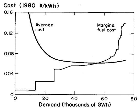
4.1. 1980 Marginal and average cost curves.

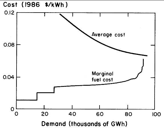
4.2. 1986 Marginal and average cost curves.

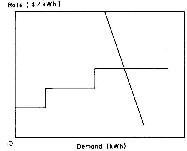
4.3. Tariff structure.

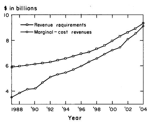
4.4. Revenue requirements and revenues from marginal-cost pricing.

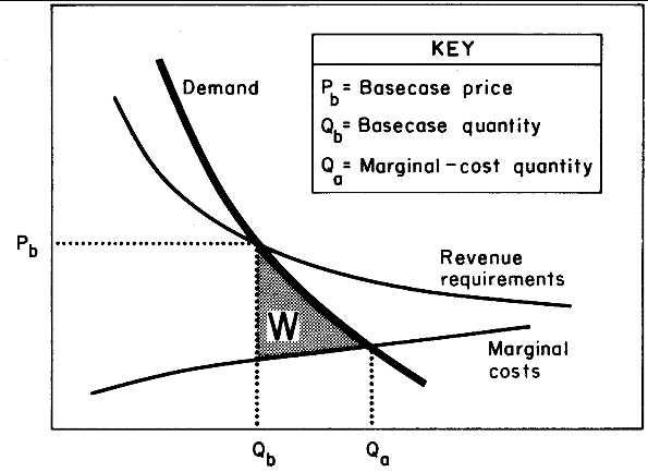
4.5. Economic gain from marginal-cost pricing.

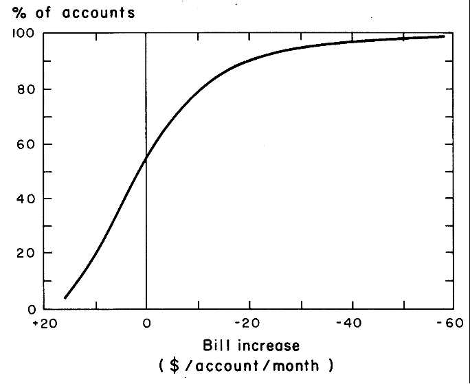
4.6. Impact of alternative rate structure: cumulative distribution (1987).

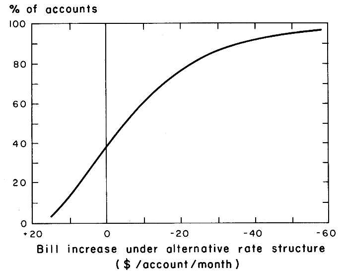
4.7. Alternative vs, CPUC rate structure.