TWO
Energy Utility Pricing and Customer Response The Recent Record in California

Lee S. Friedman

I. INTRODUCTION

This chapter surveys a variety of ideas and policy reforms concerning consumer demand for utility-provided energy. The focus is primarily on pricing policies and how they affect demand. Evaluative discussion relies on traditional economic criteria. However, in the discussion special analytic emphasis is placed on the importance of understanding actual consumer responses to complex decision problems and political and organizational constraints faced by policy makers. Data and examples are drawn largely from electric utilities in California, with emphasis on the regulatory role of the California Public Utilities Commission (CPUC).

The chapter is organized as follows. First, I briefly review some general aspects of consumer demand for energy, the institutional setting for its regulation, and the economic criteria used to evaluate pricing policies. Then I describe the process of rate setting in California and the actors involved. The description emphasizes the limited attention given to economic reasoning in the regulatory process. I conclude that the nature of this process leaves considerable room for the acceptance of economic analysis, provided that its implementation is not too complex.

I then examine recent policies for rate structure in California and proposals for their reform. These policies include the method of reve-

nue allocation and the use of charges for maximum instantaneous demand within a month, time-of-use (TOU) prices, and prices that vary with service reliability. In each case, the complexity of the customer's decision problem is considered as a factor in evaluating proposed reforms. A final section provides a summary and conclusions.

II. PRICING UTILITY-SUPPLIED ENERGY: THE INSTITUTIONAL SETTING AND ECONOMIC CRITERIA

There is a great public interest in understanding and regulating consumer demands for energy resources. In this age of heightened environmental sensitivity, it is easy to see the reason for this interest. The demands of consumers for electricity and natural gas influence the rate at which we use up exhaustible resources, such as oil (to fuel power plants) and wilderness areas with rivers (to build new sources of hydroelectric power). They influence our perceived needs for using controversial technologies, such as nuclear generating plants. Energy demands are important because of their primary functions: their uses for basic heating and cooling influence our health and our comfort at home and at work, and their uses within firms influence the cost and composition of goods and services produced in the economy and thus our overall economic well-being. If the public interest is to be served, it is important that our energy policies be as rational as possible.

To understand the policy issues that arise in energy pricing, one must have a sense of the institutional settings in which policies are formulated, debated, and implemented. Energy utilities in the United States virtually always operate under one of two types of institutional arrangement: (1) a privately owned company the retail rates of which are regulated by a public utilities commission (PUC) or (2) a publicly owned and operated enterprise. In either case, the public sector has direct and continual responsibilities for the setting of utility prices. The analysis of rate design issues I shall be discussing applies generally to both institutional arrangements, because the public sector powers and responsibilities are similar.^[1]

The primary reason for the particular institutional arrangements that characterize energy provision is that the technical features of the energy distribution system make it a natural monopoly. It is not sensible to have more than one set of electric wires or natural gas pipes distributing

[1] The behavior of energy utilities may vary systematically by institutional structure. The publicly owned utilities, for example, often set relatively low prices because they are financed, in part, through tax-exempt municipal bonds, which keep their capital costs low.

energy to particular physical locations.^[2] However, if there is only one private profit-seeking supplier to serve customers in the area, with neither competition from alternative suppliers nor regulation by the public sector, what forces would act to prevent monopolistic price gouging and service of poor quality or inadequate quantity? Thus energy utilities have historically been regulated or operated by the public sector, as have providers of local telephone service and water.

Traditionally, public sector officials have emphasized the need for equitable prices. Various conceptions of equity may underlie different aspects of ratemaking. For example, virtually every state PUC limits the total revenues collected by a utility to consist of operating costs plus a normal profit (a "fair" rate of return on capital). In recent years a small number of states have adopted explicit policies to ensure that some minimal level of energy is available at a subsidized rate to some or all residential customers. State PUCs also have responsibility for the efficiency with which scarce energy resources are used, and in recent years attention to this aspect of energy regulation has been growing.

When economists have analyzed local power provision, they have always used one key principle in their pricing recommendations: prices should be based on marginal opportunity costs. The opportunity cost refers to the value of the resources used to provide a service in their best alternative uses. If a price is set equal to the marginal opportunity cost of supplying a service, then, in effect, every potential consumer is encouraged to consider whether the benefits of additional consumption are greater or less than the costs in terms of foregone benefits from the best alternative use. If all customers perceive this and respond in a fully knowledgeable way, they will only consume those quantities for which the benefits outweigh the costs. This will result in the allocation of resources to their most highly valued uses; such an allocation is called efficient .

In fact, it is much simpler to advocate the use of theoretical principles than it is to achieve their implementation. Important real-world complexities, which theory often assumes away, must be faced. Thus perhaps it is not surprising that in the United States today only a handful of state PUCs (such as those in California, Oregon, New York, and Wisconsin) have embraced marginal-cost-based pricing principles. We shall use California as a case study of the progress made and problems encountered.

The CPUC first made explicit reference to marginal costs in rate design in 1979 (Parry, 1984). In its decisions it has indicated a rationale for using marginal costs virtually identical to the social objectives stated above: "The result of basing rates on marginal costs is that . . . each consumer pays the resource cost . . . Conservation is achieved since con-

[2] For some customers, self-generation of energy may provide a viable substitute. But these are exceptions.

sumption is made only when the benefits of consumption are greater than or equal to the cost . . . Efficiency is achieved since the least-cost combination of resources neither overuses the good nor underuses the good . . . Finally equity is achieved since no customer underpays relative to the resource cost" (California Public Utilities Commission, 1980, p. 10).

These laudable goals have been subservient to the objective of total cost recovery in utility ratemaking. The CPUC did not intend to set consumer prices equal to the marginal cost of providing utility service to the customer. Rather, the CPUC designed a formula using marginal-cost estimates to allocate the total cost of utility services to different customers such that each customer pays a rate that is a multiple of the marginal cost of serving that customer, with the same multiple for every customer. This is known as "equal-percentage of marginal cost" (EPMC) ratemaking. When the average cost of service differs from the customer's marginal cost, EPMC rates also differ from the marginal cost of service.

Notwithstanding the fact that EPMC ratemaking is only a partial move toward the principle of setting rates equal to marginal cost, progress in this direction has been impeded by other considerations. In general rate cases involving the Pacific Gas and Electric Company (PG&E) (1984) and the Southern California Edison Company (SCE) (1985), the CPUC chose to weight the revenue allocation among customer classes (residential, commercial, industrial) by only 5% based on marginal-cost considerations (EPMC) and 95% based on historical allocations.^[3] In other areas as well, the CPUC approves rates that depart significantly from those based on marginal costs. What is preventing, or retarding, more extensive use of marginal-cost principles? I shall consider and illustrate this shortly by examining several of the rate design questions at issue in a CPUC general rate case.

Most theoretical studies assume only a few prices to be set. But in actual practice utilities sell a large number of services and must set a price for each. For example, SCE has 49 different rate schedules for electricity sales (varying by the type of customer and service provided), each with between three and eight price components. Thus the CPUC must set hundreds of prices for just this one utility. Other utilities sell both electricity and natural gas and have even more rate schedules. The entire set of utility prices is referred to as the rate structure. Each component of the rate structure must be determined so that the revenues raised overall lead to the allowed profits. This complexity complicates considerably the

[3] On the other hand, the CPUC relied completely on the EPMC methodology for its revenue allocation in the most recent general rate case for the San Diego Gas and Electric Company (1983).

price-setting process. To consider the use of marginal-cost principles to determine the rate structure, it is useful to review its components.

Energy prices are set separately for the major classes of energy customers: residential, commercial, and industrial. Within any class of customers, price may vary by season and by time of day (e.g., peak load pricing), by the quantity purchased (e.g., connection charges, baseline or lifeline tier quantities), by the instantaneous speed or flow of delivery of the quantity (demand or maximum kilowatt charges), and by the quality in terms of reliability of the service purchased (interruptible contracts or direct load management services). Thus many rate schedules apply within a customer class, depending on the specific type of service a particular customer receives. A question of equity that typically arises in regulatory proceedings and constrains the prices in specific schedules concerns the proportion of total revenue that is raised from each major customer group; this is referred to as the class allocation issue.

Marginal-cost principles can be used to guide pricing of each component of the rate structure. The key question is whether each customer perceives the appropriate price for marginal changes in his consumption. Because the actual marginal cost varies substantially, depending on such factors as the time the service is demanded or the reliability of the service promised, the presumption is that the rate schedule should reflect these variations. Several of the ideas discussed in the literature, such as peak load pricing (also called time-of-day [TOD] and time-of-use [TOU] pricing) and interruptible contracts, have been tried as experiments or are used to a limited extent. However, many of these ideas have not received the widespread acceptance originally hoped for by their proponents. I shall consider the obstacles to their fuller implementation.

The next section reviews the actors involved in California rate setting and the process used to determine rates. Such review helps identify Political forces and organizational capabilities that constrain the use of marginal-cost pricing principles to achieve equity and efficiency objectives.

III. THE PRACTICE OF ENERGY UTILITY POLICY MAKING IN CALIFORNIA

In most respects, the institutional structure for regulating power utilities in California is similar to that used in other states. The CPUC is responsible for regulating the rates charged by private utility companies to their customers. Unlike most other states, California has a separate body, the California Energy Commission (CEC), which has regulatory

authority over utility requests to add new power sources. Because this chapter focuses on the rate-setting process, I will concentrate on the CPUC.

Every three years, each private utility initiates a general rate case.^[4] The utility requests authorization from the CPUC to charge particular rates, and the requests are analyzed and considered in a quasi-judicial process that takes about 14 months. Between general rate cases, rate adjustments are allowed through frequent "offset" rate proceedings. Offset proceedings are intended to adjust rates and revenues in response to changes in a utility's costs that are beyond management control. These costs are principally for fuel, and changes are largely based on the application of preexisting fuel adjustment clauses. Offset cases do not generally result in major policy changes.

The main issues of rate design are considered in the general rate cases. These cases have three stages: analysis, hearings, and decision making.^[5] CPUC staff analysis begins when the utility files a Notice of Intent to apply for rate changes, along with draft versions of its supporting testimony. Individual staff members from the CPUC Rate Design Branch are appointed to analyze the utility's rate structure proposal, and the commission selects one of its five members to oversee the case and appoints an administrative law judge to conduct the hearings.

About two months after the Notice of Intent is filed, the utility formally files its rate change application and submits final versions of its supporting arguments. The CPUC staff then has about three months to analyze the request and prepare its response and rate change proposals. Then the hearings begin. Testimony is given, with all parties (utilities, CPUC staff, and interest groups) represented by lawyers who can cross-examine witnesses. The hearings themselves usually last four or five months, and the presiding administrative law judge issues a draft decision about two months after the hearings are concluded.

The final stage of decision making begins with the issuance of the draft decision. The draft is circulated to the commissioners and senior staff, and within the next month oral arguments are formally presented to them by the parties to the case. Then the informal process of building consensus among the commissioners for an amended decision occurs, and the final decision is usually issued about two months after the start of this stage.

Substantively, each case proceeds in the same way. First, the utility's revenue requirement and marginal costs are determined. Second, the

[4] Until recently, the general rate cases were held every two years.

[5] Much of the following information is drawn from Hausker 0985).

commission comes to a broad decision about how to allocate that revenue among customer classes. Finally, actual rates within classes are set to raise the allotted revenue. However, a closer look at the process reveals important constraints not seen by considerations of substance alone. The logic in decision making is strongly influenced by the CPUC organizational routines, as well as the backgrounds of the individuals from the CPUC involved in the case.

About 20 staff members comprise the Rate Design Branch, with about two-thirds working on electricity issues and the rest working on natural gas. By training, roughly half have engineering backgrounds with a few economists, statisticians, business administrators and others comprising the balance. In making recommendations, the staff usually follows precedent from past cases. There are several important reasons for this. It eases the staffs heavy work load. Because the administrative law judges and the commissioners strongly attend to precedent in their reviews, following precedent is most likely to be acceptable to them. Acceptability is itself important in CPUC evaluation of the work of the Rate Design Branch. In addition, following precedent will result in fewer requests for additional work in the later stages of a rate case.

Another reason for often following precedent is that the staff typically lack the information necessary to apply innovative designs, such as those based on recent theoretical work in economics utilizing marginal-cost principles. Most of the Rate Design staff are unfamiliar with theoretical concepts such as optimal nonlinear pricing.^[6] The few economists on the staff have never attempted to apply any of the more sophisticated concepts from welfare economics to a specific electric rate design.

Furthermore, even if the staff were more inclined to apply such ideas, it does not generally have the necessary empirical information. For example, these ideas usually require knowledge of price responsiveness of the specific consumers affected by the design. But the Rate Design Branch only has a fixed sales estimate as input with which to work. The latter implies the false assumption of zero price responsiveness, but it has the great virtue Of simplicity and easy availability. These reasons explain why the Rate Design Branch usually follows precedent, although there are exceptions.^[7]

The next organizational layer, the administrative law judges, adhere even more strongly to precedent. Most of the administrative law judges are lawyers, although some are engineers. Lawyers are, of course, highly

[6] This concept is discussed later in the chapter. Note that more expertise with concepts of welfare economics could be obtained by having more economists on the staff. However, one should keep in mind that economists generally have little or none of the engineering skills useful in rate design, and the optimal staff composition is not obvious.

[7] For more detailed discussions of the exceptions, see Hausker (1985, Chapter 7).

trained to attend to precedent. Furthermore, because these individuals are generalists who must deal with all aspects of rate cases, they are less familiar with the details of analytic methodologies applied to specific issues in a case. They are more comfortable checking arguments for consistency with prior decisions than making decisions on methodological grounds, such as those involving sophisticated economic reasoning.

In the final decision-making phase of the case, the role of the commissioners themselves takes on a great importance. The commissioners are not elected officials but are appointed by the governor for six-year terms. They rarely come to the job with experience in public utility regulation or knowledge of economics, and they are almost never reappointed. They generally see their role as one of avoiding "unfair" rate design. They check the rate design by eyeballing tables of numbers reflecting class allocations and residential rates. The underlying rationales for these numbers are not too important to them; significant departures from the outcomes of the current rate structure are. They demand repeated iterations of the numbers to see the effect of certain changes.

Because the commission often makes none of the major substantive decisions in the case until the final weeks, myriad frantic recalculations are typically necessary as the commission tries to reconcile modifications to one part with their implications elsewhere. For example, commissioners often do not decide the total revenue requirement until the last minute, which requires a revised class allocation decision and then recalculation of all specific components of the rate design. Thus the latter must be easily and quickly alterable to meet the overall requirement.

Naturally the utility being regulated fights hard for its positions throughout this process. However, the offset policies mentioned earlier have the effect of reducing the utility's stake in rate design. In particular, the energy rate adjustment mechanism (ERAM) insulates the utility on the revenue side, and the energy cost adjustment clause (ECAC) insulates it against changes in fuel costs. Both mechanisms provide for adjustments in the per-kilowatthour rates to ensure the collection of the forecasted (and CPUC approved) total revenues as well as to adjust for any differences between forecasted and actual fuel costs.

Except for administrative and other nonfuel operating costs, these clauses guarantee the dollar return to the utility specified in the general rate case. Thus unanticipated revenue and fuel cost effects of specific changes in the rate design (e.g., increased use of TOU rates) are eliminated by the adjustments. Although these clauses mitigate utility concern over rate design changes, they do not eliminate that concern. The utilities still prefer not to change the design if they think the change will confuse customers and create complaints. However, the clauses minimize utility opposition to rate design changes and thus enhance

the ability of the CPUC to experiment with marginal-cost-based pricing principles.^[8]

To sum up this discussion, the process of deciding a general rate case reveals important constraints not seen by considerations of the substance alone. The economist interested in the increased use of marginal-cost-based principles must keep several ideas in mind. To increase chances for adoption, four characteristics are desirable for any new method of rate design. One is that it should be simple to calculate and should require only information that is already available or easily obtainable. Two is that it should be simple to explain to noneconomists, particularly the extent to which it utilizes principles acknowledged in prior decisions (and thus can be seen to have precedent). Three is that its distributional effects on consumers (particularly across recognized classes of consumers) should be minimal. Four, it should be easily understood by consumers. This last point is given more extended discussion in the following section.

IV. CONSUMER DEMAND FOR UTILITY-SUPPLIED ENERGY

Customer demands for utility-supplied energy are called derived demands: customers (whether residential, commercial, or industrial) are generally interested not in the energy per se, but in the services that use energy (e.g., lighting, heating, cooling). That is, the customers' demands for energy are derived from their demands for energy-using services. Many factors influence the derived demands for energy. It is useful to divide these factors into two broad categories: exogenous factors, which individual customers do not control, primarily technology and prices, and customer decision making in light of the exogenous factors.

The exogenous factors determine the options customers face for obtaining the (energy-using) services they seek. For example, the energy demanded by customers for the purpose of cooling a building depends on how much energy is used by the various air conditioners available on the market, as well as the availability and attributes of such alternatives

[8] Whether or not these clauses are desirable for reasons other than easing the transition to a marginal-cost-based rate design is questionable. Essentially, they shift the risk from factors beyond the utility's control (such as weather, general economic conditions, and unanticipated consumer responses to CPUC-mandated rate designs) away from the utility and onto its customers. This shift lowers the interest rate the utility must pay to borrow funds (and reduces the risk to its stockholders), but it makes all customers feel worse off because they bear increased risk. Although this issue is a difficult one to resolve empirically, efficiency requires that risk be borne by the agent who has the least cost of bearing it. If the extra risk cost to consumers from each of these clauses exceeds the savings to the utility from its reduced capital costs, then they should be eliminated eventually.

as thermal coating of windows or other insulating measures. The climate is another important exogenous factor. For buildings that already exist, the climate is determined by location. If constructing a new building, however, a customer may choose from among a variety of climates by deciding on a location.

Customer choice from among the available options depends on knowledge, preferences, and budget constraints.^[9] Knowledge refers to the customer's understanding of the various attributes of each alternative. For example, does the customer know how much energy a particular air conditioner will consume when operated, and does the customer know how much this energy will cost over the life of the air conditioner? Does the customer know how to translate future costs into present-value terms? Does the customer know about alternatives, such as thermal coated windows? Does the customer know how energy costs are affected by building or plant location in a hot region or a moderate one, even within a metropolitan area near a windy shore or a sheltered site inland? When making choices, some customers may have much more information than others faced with comparable choices and may use it more effectively.

In light of the customer's actual knowledge, choice still depends on the customer's preferences and budget constraints. To continue with the cooling example, the customer may have limited space for an air conditioner and therefore may seek a relatively compact one. Or a customer may seek an air conditioner that is unusually quiet. The residential customer may know about thermal window coatings but may not like their aesthetic effects. The industrial customer may know how much greater energy costs are in a southern location, but the quality of the available work force may be more important. Finally, the customer must reconcile preferences with economic means. Not everyone can afford a deluxe model air conditioner, and the purchase choice will reflect the customer's budget constraint.

These examples suggest the following points. We know from basic economics that energy prices are factors in customer decisions about how much energy to demand. However, in many cases prices may be minor factors compared with other attributes of the energy-using services customers seek. In making their decisions, fully informed consumers may consider extensively the consequences of energy prices.

[9] The customers of utility companies consist of households and firms. In economic theory, preferences and budget constraints are attributes of consumers seeking to maximize utility. Although households are typically treated as this type of economic agent, firms are generally modeled as seeking to maximize profit. For simplicity, the above discussion does not make this distinction and describes all customers with the language for consumer choice. The behavioral points made are valid for firms as well as households.

Neverthless, in these cases, other factors may matter much more. In addition, many other customers may-perceive only dimly at best the consequences of energy prices for their decisions. In these latter cases, the effects of energy prices may be more difficult to analyze.

Public policy can affect the demand for utility-supplied energy through the use of diverse instruments. Prices can be lowered or raised to encourage or discourage the purchase of particular goods or services. Regulatory restrictions can be used to limit the range of options available to the consumer. Educational efforts can be undertaken to alter consumer choices from the available options. These actions can affect customer decisions directly, as well as indirectly, by causing changes in the available technologies for energy-using services.

Much of the rationale for policies involving regulatory restrictions and educational efforts depends on the assumed existence of important imperfections in the consumer decision-making process. To the extent that these imperfections are present, they may also affect pricing recommendations. Let us consider as an example technological regulations. These are restrictions that limit the choice of options available to consumers. Energy efficiency standards for refrigerators or required conservation measures in new homes and buildings affect demand by restricting the available options for energy-using appliances and structures. That is, these regulations are choice restrictions because they ban the sale of products (refrigerators and new homes) that do not meet the standards.

What is the rationale for such standards? Obviously the regulators must think that without the regulations too many refrigerators of the energy-hogging type are bought and too few conservation measures are installed in buildings. Do the regulators have different objectives than the consumers? According to the reports of the CEC, this is not the reason for such regulations in California. Rather, the CEC relies on the idea that many consumers will not be aware of the energy-cost implications of purchasing unregulated appliances or buildings and thus not act in their own best interests.^[10] If consumers only lack information, why not solve the problem through educational efforts rather than regulations? To this idea the commission responds by citing the difficulty and great expense of educating consumers and states "there are cases where it costs less to install measures for free than to provide information to consumers" (California Energy Commission 1983, p. 126).

[10] The commission also argues that imperfections in capital markets will leave some consumers unable to finance conservation measures that save them money in the long run through lower utility bills. However, regulations banning the alternatives with lower initial costs do nothing to make the remaining unbanned alternatives with higher initial costs more affordable. Thus imperfect capital markets are not a rationale for the types of regulation we are discussing. See California Energy Commission (1983), pp. 124-126.

Based on the studies available, the CEC appears to be on solid ground in its claim that energy consumers often do not act in their own best interests. According to evidence summarized by Stern, "people tend to overestimate the amounts of energy used by . . . technologies that must be activated each time they are used. Thus people overestimate energy use by televisions and lights and underestimate energy use by furnaces and water heaters . . . to save energy they will do more light dousing and less furnace retrofitting than is in their economic self-interest" (Stern, 1986, p. 205).

Furthermore, there is often little or no effect of providing information to consumers in the hope of inducing them to act in their own self-interest. Numerous factors explain this disappointing result. First, the information may be ignored if it is only relevant to a calculation the consumer does not know how to make. In a study of disaster insurance purchases, Kunreuther (1976) found many consumers who had no notion of expected-value calculations and thus no response to information about damage probabilities. With respect to energy consumption, consumers who have no notion of present-value calculations may ignore information about future energy prices.

Second, the form of the information matters a great deal. In one study, consumers receiving a carefully designed package of information cut energy use in response to TOU energy rates by 16% compared with a control group receiving the sponsoring utility company's standard information package (Heberlein and Baumgartner, 1985; cited in Stern, 1986, pp. 205-206). In another study, the best-designed information package increased the average efficiency of a household's choice to 51% from the 43% based on the standard utility-provided package; this example illustrates that even the best information efforts still result in large numbers of consumers making choices substantially worse than their optimal ones (Magat, Payne, and Brucato, 1986).^[11]

Finally, the source of the information, particularly its trustworthiness, also matters to consumers. Two groups of energy consumers in New York State were sent conservation brochures that were identical except for the letterhead. The group receiving the brochure with the letterhead of the New York State Public Service Commission cut energy by 7% in the following month, compared with no reduction from the group receiving the brochure with the letterhead of Consolidated Edison. In another study, a county government with no energy expertise was five times as effective as an energy company in enrolling participants in the same home retrofit program offered at no cost to participants. In both cases, the difference was attributed to the differential trust consumers

[11] The study is based on a laboratory experiment in which the most efficient household choices were controlled by design.

had for the respective information sources (Craig and McCann, 1979; Miller and Ford, 1985; both discussed in Stern, 1986, p. 206). These studies also help explain why consumers often rely on the advice of non-expert friends while ignoring the advice of experts.

One of the missing pieces of information to many consumers may be the price of energy.^[12] To continue with the example of an air conditioner purchase, a customer should know not only current but future energy prices. That is, it is not enough to know how much electricity the air conditioner will use, but how much will be charged for that electricity, which depends on the price of electricity over the life of the air conditioner.

Figure 2.1 illustrates in one simple way why prices may be difficult to perceive. Imagine the following scenario, which is like the position of electric utilities with excess capacity in the late 1970s and early 1980s. Let De be the electricity demand originally expected by planners,^[13] and let the long-run marginal cost per unit including capacity be Q_E These parameters lead planners to provide a capacity of Q _C , where the demand and long-run marginal-cost lines intersect. However, actual demand turns out to be D_A and if price P_E were charged, only Q_A units would be demanded and there would be much unused capacity in the system. Therefore price is set in the short run at P_A , which makes the actual demand fully utilize the available capacity.^[14]

In this scenario consumers are currently facing a price of P_A per unit of electricity. However, suppose planners expect (more reliably this time) system demand to grow over the next few years to D_F . Then, the utility will have to add new capacity (to Q_F ) and in the future charge price P_E .^[15] The question is, if you are the consumer deciding on an air conditioner purchase today, what assumptions about future energy prices will you be

[12] For evidence and discussion of this point, see Stern (1986), Quigley (1986), Friedman and Hausker (1984), and Kempton and Montgomery (1982).

[13] By planners, I am referring to the technical staff of utility companies and regulatory agencies with extensive resources for econometric forecasting. Although the accuracy of any forecast is always uncertain, I am assuming that better forecasts can be produced when more resources are put into the forecasting effort. That is why I assume planners make better forecasts of future prices than average consumers.<HR>

It also should be noted that utility companies and regulatory agencies may have reasons to bias their forecasts. My impression from examining demand forecasts made by Califor-nia utility companies and by the CEC is that some biases do exist but that they tend to be offsetting.

[14] This is the price at which the short-run marginal-cost curve SMC(Q_C ) intersects the actual demand curve. The short-run marginal-cost curve typically consists of two segments: a horizontal segment with height equal to the marginal operating costs for any quantity up to the system capacity, and a vertical segment when system capacity is reached.

[15] Note that P_F . is again the price at which the short-run marginal-cost curve intersects the demand curve. The additional capacity causes the short-run marginal-cost curve to shift from SMC(Q_C ) to SMC(Q_F ).

making? It is quite plausible that many consumers are myopic and only consider the current price. They will act as if future prices will be close to P_A , despite the much higher likelihood that they will be close to P_E .

This raises the following interesting policy question. If all consumers have correct perceptions of current and expected future energy prices P_A and P_E (as well as of other decision factors), then they will make both short-run and long-run energy consumption decisions that are in their own best interests. Suppose, however, that a certain portion of consumers are myopic in the manner suggested above, and suppose further that there is no inexpensive way of correcting their expectations.^[16] Is there some way that policymakers can take account of this behavior? For example, might it be better to make the current price equal to P_E ? Then there would be no long-run mistakes due to myopia. However, this policy comes with a disadvantage that is likely to be substantial: it would cause too little consumption (Q_A ) in the short run. (Q_C is the most efficient short-run consumption level.) Using traditional economic logic, one could ask whether the efficiency losses from the short-run misallocation with high excess capacity (shown as the shaded area in Figure 2.1) would be offset by the gains from better consumer decisions having long-run consequences. If so, then it would be better (on efficiency grounds) to make P_E the current price. This scenario illustrates how the existence of imperfections in consumer decision making can affect pricing recommendations.^[17]

The above example does not imply that an appropriate response to imperfect consumer decision making is to price at long-run marginal cost. As mentioned, it is not the least bit clear that the long-run gains would outweigh the short-run losses. Even if they did, there are other alternatives that retain pricing at short-run marginal-cost and that are likely to be more efficient. Consider whether the technological regulations with which we began this example combined with the use of the price P_A currently might not be a better policy package than simply using P_E for both current and future prices. The answer is probably yes. The policy of regulating technology avoids the short-run misallocations caused by making the current price equal to P_E . However, it will yield somewhat smaller long-run gains.

[16] That is, an attempt to "inform" consumers by, say, including the future price information in a current mailing does not work for the general reasons discussed earlier: many consumers will not read the information; others will not trust it or will forget it; and still others will ignore it because they do not make decisions by making present-value calculations as explained in economics textbooks.

[17] As an empirical matter, it is probably true that even long-run marginal cost is substantially lower than the current prices faced by California consumers. See Chapters 4 and 6 in this volume.

The regulatory policy will prevent many long-run mistakes that myopic consumers would make, e.g., the purchase of energy-hogging types of regulated appliances and buildings by consumers who underestimate their operating costs. However, not all long-run consumer decisions can be regulated, so some long-run errors would persist. Furthermore, a new type of consumer mistake is caused by the technological regulation. Some nonmyopic consumers might wish to purchase the banned appliances considered inefficient by the regulators, and thus the regulations would cause these consumers to be made worse off. Should this latter group be large, the technological regulations could actually worsen the long-run decisions on balance (compared with no technological regulations, other things equal). Even if this latter group is small, some long-run consumer decisions will be faulty under the regulatory policy. On the other hand, the policy of making current price P_E leads to no long-run errors. Nevertheless, the substantial short-run advantage of the technology-regulating approach is likely to outweigh its long-run disadvantage. Thus in the absence of convincing empirical information to the contrary, the standard recommendation to price in accordance with short-run marginal costs will be maintained in this analysis.

The discussion of this section has emphasized the importance of understanding actual consumer decision making in order to link public policies to their energy-consumption and efficiency consequences. The issue of actual consumer behavior and the clarity of price signals will arise again in the discussion of what it means to implement pricing at short-run marginal cost in the form of an actual complex rate structure.

V. REVENUE ALLOCATION

The rate design decisions made in the general rate cases start after the marginal costs have been estimated and the total allowed revenue to the utility decided. One interesting and important aspect of these prior decisions as well as of those to follow is that, as mentioned earlier, to make them the CPUC (like most state commissions) works with a fixed estimate of expected sales. This means that no matter how the rest of the rate structure is decided, it must have the characteristic that the final rates applied to the fixed sales estimate add up to the total allowed revenue. It also means that the final rates applied to the fixed sales estimate for each customer class must sum to the revenue allocation for that customer class. This constraint of a fixed sales estimate seems to ignore basic economics: quantity purchased will depend on the price.

The basic rationale for the constraint is to simplify the decision process. If quantity estimates were allowed to vary with specific rate propos-

als, then all parties to the case would have to have estimates of the price responsiveness of each customer class to each of the rates that it faced (e.g., peak time, midpeak and off-peak price elasticities of SCE's large industrial customers with automatic powershift, and estimates for the same elasticities for those large industrial customers without automatic powershifting, and the price elasticity of the powershift option itself). We have already mentioned that this information, for the most part, does not exist. This would leave the CPUC in the position of having to pick from among the large array of estimates and guesses offered by the different parties to the case, with very little knowledge to form a basis for its decision.

Similarly, the fixed marginal-cost estimates seem to defy economic logic: marginal costs will depend on the quantities of energy bought under a specific rate structure. Yet the economic errors that arise from both of these simplifying assumptions are probably small. Because the demand for energy is highly inelastic in the short run and the marginal-cost curves are likely to be relatively flat over the small range of plausible short-run quantity variations, the simplifying assumptions should not cause large differences between the estimates and actual quantities and marginal costs.^[18] Furthermore, if one envisions an iterative adjustment process of the sales forecast from one rate case to the next, earlier forecast errors can be corrected over time.^[19]

How should the CPUC proceed in making its revenue allocation decision? If we turn to economic theory for normative guidance, we may be struck at first by the inattention to this decision. Normative economic theory is, for the most part, concerned with the derivation of the most efficient prices given the total revenue constraint. Use of the most efficient prices implies the revenue raised from each customer class; no further decisions are necessary.

Three different approaches to calculating the most efficient prices are found in the economic literature: optimal nonlinear pricing, optimal uniform pricing, and the two-part tariff. Collectively, these approaches are generally referred to as second-best pricing principles. They are called second-best in recognition that the best pricing principle— pricing each customer class at its marginal cost—is infeasible because it would violate the overall profit constraint.

[18] Although rapid changes in fuel costs can occur and result in substantial marginal-cost changes, they are handled through the offset clauses mentioned earlier. Our interest here is whether any errors in quantity forecasts can themselves be the cause of substantial errors in marginal-cost estimates.

[19] See Manski (1979) and Willig and Bailey (1979) for analysis of adjustment rules to use as a response to limited empirical information.

For example, in the 1985 SCE general rate case, marginal costs were estimated as substantially greater than average costs.^[20] The estimated revenue produced by marginal-cost pricing would have been $5.34 billion, whereas the allowed revenue was only $4.80 billion and included allowance for a 16% rate of return on common equity capital. Marginal-cost pricing would have led to an overall rate of return on equity capital of 39%!^[21]

A brief review of the three different methods in light of the organizational and behavioral constraints I have previously identified will help to identify promising approaches. Historically, the principles for optimal uniform pricing under a profit constraint were developed first, and we begin with consideration of its potential for practical application to rate design.^[22] Uniform pricing is this context means that the price per unit to a customer is the same regardless of the quantity of units purchased (i.e., there are no block rates).

Optimal Uniform Pricing

No Utility Applications. To my knowledge, no utility or its regulatory commission has ever attempted explicit use of the principles for optimal uniform pricing. These principles, often referred to as Ramsey pricing and the inverse elasticity rule, require knowledge of the elasticities of demand for each product to be priced. They do not themselves provide guidance on what products should be priced separately (nor do any of the other methods I discuss)^[23] If we accept for the most part that utilities will continue to establish separate markets for residential, commercial, industrial, and agricultural customers and will have multiple products within each class (e.g., rates that vary by time of use, connection charges, etc.), then quite detailed knowledge of the elasticities is required for application of the rules for optimal uniform pricing.

I have already mentioned that utilities and their regulatory commissions do not generally have the necessary information about the elasticities specific to their customer markets. Furthermore, there may be legal

[20] Other chapters in this book suggest that California is about to enter an extended era where the marginal costs of electricity production are below average costs.

[21] The total SCE rate base was $5.13 billion apportioned 45% to common stock equity, 10% to preferred stock, and 45% to debt. The net revenue allowed SCE was $652 billion, of which $370 billion was the return to common equity. The extra revenues from marginal-cost pricing would increase this return to $910 billion or 39.4% of common equity. See California Public Utilities Commission (1984), Appendix B, p. 39.

[22] The first statement of these principles is Ramsey (1927).

[23] If the sole objective is economic efficiency, then one segments the market (i.e., sets a separate price) to minimize any deadweight loss caused by the profit constraint. Deadweight loss is a measure of the magnitude of the efficiency decrease. For an exposition of such measures, see Friedman (1984), Chapters 5 and 7. In special cases, the second-best prices may result in no deadweight loss.

constraints on this type of pricing. The U.S. Postal Service explicitly used these principles in the early 1970s, but this use was struck down as discriminatory in the U.S. Court of Appeals for the District of Columbia Circuit (Tye, 1983). Thus the obstacles to the use of this method are considerable.

The EPMC Method as an Approximation. Nevertheless, some work has been done in an attempt to devise an easily implementable decision routine that approximates the optimal uniform prices. Hausker (1985), for example, has shown that under certain conditions likely to apply to the allocation problem across customer classes, setting prices for each customer class at an equal percentage of class marginal costs (a rule that is very simple to implement) gives a solution close to the efficiency level of the optimal uniform prices.^[24] A particularly interesting aspect of Hausker's work, for our purposes, is that the CPUC actually does calculate the class revenue allocations that would result from using the equal percentage of marginal cost (EPMC) method. In the case of the San Diego Gas & Electric Company, the CPUC adopted this allocation. But when the same calculations were made for PG&E and SCE, the CPUC did not like the results. In the latter two cases, the results would have been to increase substantially the energy bills of residential households. To quote directly from the SCE decision: "As in the case of PG&E, we are concerned that a significant and disproportionate increase in electric bills would result for Edison's residential customers if we were to adopt a full EPMC revenue allocation at this time…. For these reasons, we will adopt a 95% SAPC [system average percentage change, based on historical rates]—5% EPMC revenue allocation method" (California Public Utilities Commission, 1984, pp. 270-271).

CPUC Reluctance to Rely on EPMC. Curiously, the CPUC went on to assert that "this is consistent with our policy . . . of moving towards a full EPMC revenue allocation method" (California Public Utilities Commission, 1984, pp. 270-271). It is clear, however, that the CPUC is substantially more interested in protecting the residential class from rate increases than it is in achieving efficient allocations. There can be multiple

[24] The important condition, stated as a rule of thumb, is that the price elasticity of demand for any particular class be leas than twice the price elasticity for any other customer class. However, establishing the efficiency level of an actual rate structure is more complex than assumed in the calculation. The "price" per customer class used is actually not a price. It is the weighted average of the different lower-level prices that are yet to be set (e.g., peak, midpeak, and off-peak prices faced by industrial customers). Actual efficiency depends on the specific prices used in the rate structure, and is not simply a weighted average of them. This point is illustrated later on in the text.

explanations for this behavior: the political clout of the residential class compared with that of commercial or industrial customers, a genuine feeling on the part of the CPUC that equity requires residential customers to be subsidized at the expense of other customers, or a belief that rate stability is important per se. Let us comment briefly on these different motives.

Residential customers possibly exert more effective pressure on the CPUC than do business customers; however, not at the staff level. In both the PG&E and SCE cases, the CPUC staff recommended class allocations much closer to the EPMC allocations than those the commissioners ordered. Thus the rationale of the commissioners themselves (and their aides) must explain the decision.

At the end of their appointed terms, most commissioners move on to other state and federal government positions or retire. Political sensitivity while they are commissioners could increase their prospects for future government positions. It may be that residential customers, through their voting power and influence on elected officials, have more clout in terms of these future prospects than do business interests. But this question is an open one. Rarely is a PUC a hot topic in a campaign for governor, and business interests can be highly effective politically by hiring full-time lobbyists.^[25]

The equity rationale is an interesting one. Perhaps some people naively think that the extra charges imposed on business customers end up being borne by people who do not live in residences This, of course, is silly: extra costs to businesses are born primarily by the customers of those businesses, in part by the employees (in the form of lower wages) and in part by the owners (e.g., when there is substantial competition from out-of-state producers). It is not apparent that the burden of business energy costs is any greater to the lower-income population than are residential energy costs.^[26] Perhaps more to the point, cross-subsidization of this type is not targeted specifically to the lower-income population

[25] One study, using observations on private utility company rates from a national sample, found negligible impacts of grass roots activists on the allocation of costs between residential and business customers. This finding does not support the hypothesis that, relative to business interests, residential interests can be effectively pursued through the political process. See Gormley (1983), p. 169.

[26] One could argue that if the income elasticity of demand for residential energy is small, the lower-income population bears a proportion of residential energy costs much greater than its proportionate share of residential income. Because spending for general consumption and investment is proportionate to income, the lower-income population does better as energy costs are shifted from the residential to the business sector. However, residential energy costs may have the primary effect of reducing residential land value, and residential land is owned disproportionately by the wealthy. This would negate the argument.

at all. Despite its lack of knowledge about the true effects, the commission may believe nevertheless that equity requires subsidizing residential rates.

Rate stability per se is also an interesting possible rationale. Whatever value is placed on stability, it must not apply with the same force to the commercial and industrial classes: for a given overall change in the revenue requirement, the logical consequence of stabilizing residential rates is to cause greater instability to the commercial and industrial customers. Two different reasons might motivate the quest for residential rate stability: (1) reducing consumer hardship due to unexpectedly high bills and (2) reducing consumer difficulty with family budget planning.

Both of the above reasons rely on assumed imperfections in residential decision making: the residential customer fails to anticipate bills properly. However, this may also be a problem for commercial and industrial customers. Perhaps simple and clear advance notification of the new rates could solve this problem, although the evidence reviewed earlier on the effects of providing information to consumers does not result in optimism on this point.^[27] Given that customers have bill anticipation problems, the residential customer (relative to the business customer) might have a harder time financing large bill increases.

In summary, I have not identified clear and compelling logic to explain why the public interest is best served by GPUG decisions to deviate from the results of the EPMC calculations. However, we can understand that the CPUC may believe that the public is served by doing so, and we certainly should expect that they will continue to act in this manner. Thus even if the EPMC method could be shown to be a step toward substantial efficiency gains, the prospects for its actual implementation promise to be, at best, unduly slow and, at worst, not successful at all.

The Inefficiency of the EPMC Method. Recall the comments made earlier concerning economic theories of second-best pricing and the lack of attention to the revenue allocation decision. Assuming the CPUC did adopt the EPMC calculations for its revenue allocation decision, the efficiency of this approach cannot be evaluated without knowing the

[27] For example, each residence can be mailed a notice saying: "This is not a bill. Energy rates have had to be increased for the coming months. If your energy usage during these months is identical to the prior year, your new bill will be $__. This compares with your actual bill last year of $__. To keep your new bill as low as possible, we urge you to review the ideas in the attached pages for energy conservation. We are doing our best to keep rates as low as possible. We hope that this notice will help you to plan now for the upcoming months." <"HR>

This type of notice may not be useful for new customers who do not have a prior billing history. However, these customers have difficult planning problems whether or not rates are increased.

further details of the rate decision. If each customer class really faced a simple uniform price per kilowatthour as the only charge, then the marginal price would indeed be implicit in the EPMC revenue allocation decision. But each customer class does not and need not face such a charge.

For example, residential customers face an inverted block rate structure called baseline, in which the price per unit within the baseline quantity is lower than the price per unit for any units purchased above the baseline quantity. Table 2.1 gives the 1985 rate schedule that applied to the overwhelming bulk of SCE residential customers. One can see (from the bottom line) that the average rate is 7.87¢/kilowatthour, but the marginal rates for customers are either 6.57¢ or 9.67¢ and depend on whether they fall short of or exceed the baseline quantity.^[28]

Even if the CPUC adopts the EPMC method to set the average rate for each customer class, the method is not designed to guide the decompositions of the average rates into their components. But the fact of these decompositions affects efficiency and, in general, invalidates the basis for the original EPMC calculation. To see this, consider a simple illustrative example in which all nonresidential classes have a uniform rate equal to that calculated by the EPMC method. Thus the only decomposition required in this example is into residential baseline and nonbaseline rates.

In general, the demand for baseline electricity is more inelastic than the demand for nonbaseline electricity.^[29] But to make the example transparent, suppose the demand for baseline electricity is perfectly inelastic. Then it is more efficient to discard the original EPMC calculation across customer classes and to set all prices except for residential baseline exactly at their marginal costs. The baseline rate is then set at whatever price makes the total revenue sum to the allowed amount,^[30] Note that this rate structure cannot be reached by the EPMC method, which first sets average rates per customer class and then considers their decomposition.

[28] The only place in the table where differential rates apply to baseline and nonbaseline quantities is for the energy cost adjustment (denoted ECABF). Marginal rates were calculated by summing base energy charges (excluding minimum charges, which are not per kilowatthour), non-ECABF offset charges, and the relevant ECABF charge for baseline and nonbaseline purchases.

[29] To become a nonbaseline customer, a household must first purchase the full baseline amount. For these customers, baseline purchases are intramarginal purchases and are generally not affected by rising prices. The presence of these customers in the baseline "market" makes its demand less responsive to price changes than the demand for nonbaseline electricity.

[30] This price is below (above) marginal cost when full marginal-cost pricing raises too much (little) revenue.

The example illustrates that the existence within a customer class of specific rate structure components adversely affects the potential of the EPMC method of class allocation as a tool to foster efficiency. This does not mean the method should be dismissed out of hand. It remains to be seen whether or not there is a better method that regulators will be willing to use.

The baseline and nonbaseline prices faced by residential customers in the above example actually carry us out of the realm of "uniform" pricing and into the realm of "nonlinear" pricing. Once one recognizes that utilities may set complex block rate structures to apply to each of their customer classes, new possibilities for efficiency gains become apparent. Therefore we turn to a discussion of optimal nonlinear pricing.

Optimal Nonlinear Pricing

Nonlinear prices refer to situations in which the price per unit charged to any single customer depends on the quantity purchased by that customer.^[31] Even though these pricing systems effectively price discriminate among customers, it is not done coercively: all consumers face the same nonlinear price schedule, and they sort themselves out by their quantity choices.^[32] This is unlikely to run into legal barriers in the energy utility industry because such prices in the form of block rates have been the historical norm. In fact, their common use is an advantage: compared with the others, this method may be more acceptable in practice because it seems more familiar.

Although nonlinear prices are common in the utility industry, those in use are not derived by the application of economic theory, and there is no reason to think that they are efficient prices or even close approximations. The calculation of the most efficient nonlinear prices requires data on demand elasticities of individual customers, information that is unavailable in current regulatory proceedings and perhaps unattainable

[31] For most goods, attempts by firms to charge nonlinear prices will not be practical, because a customer who can buy additional units of the good at a low price can resell them at a profit to customers who otherwise face high prices from the firm. However, it is very difficult for customers of energy utilities to resell electricity or natural gas that has already been delivered to them. Thus nonlinear pricing schemes are feasible in this setting and, in fact, are used throughout the industry.

[32] This is most clearly noncoercive in the case in which the price decreases as quantity increases. In this case, the price schedule is equivalent to offering each customer the choice of a rate plan from a menu of various two-part tariffs available to all consumers (see Willig, 1978). However, if price increases with quantity, free choice from the corresponding menu of two-part tariffs is not equivalent: customers with low consumption would choose a tariff intended for those with higher consumption, and vice versa (see Brown and Sibley, 1986, p. 81 #6). The additional restrictions necessary to enforce choice as intended are unlikely to be considered illegal price discrimination by energy utilities, because increasing block rate structures are commonly observed.

for them even with substantial research efforts. Thus some other method of implementation must be found if the theoretical efficiency advantages of nonlinear pricing are to be realized.

Willig (1978) presents an argument for a method of nonlinear pricing that requires little data and that leads to changes from existing rate structures, which makes all affected parties better off under certain circumstances. The method does not result in the most efficient allocation possible, but it does improve resource allocation. If an improvement is actually feasible to make given the constraints of the CPUC ratemaking process, it should certainly receive careful attention.

The circumstances in which the method applies require that the existing rate structure be one of uniform rates above marginal costs or declining block rates with the price for the highest quantities above marginal cost. Such rate structures are most likely to be found in industries characterized by average costs greater than marginal costs. This characterization may well be a good one of California utilities within the next few years.^[33]

The method involves adding an additional block to the status quo rate structure with price between that of the prior block and marginal cost.^[34] The logic of this method applies almost ad infinitum: Additional blocks can always generate improvements as long as there are two or more non-homogeneous customers (i.e., customers with different preferences) on the last block.

However, this method has several problems. One is that the result of improvement for all affected parties does not generally hold when the customers are in competition with each other, as is commonly the case for firms supplied by the same energy utility (Ordover and Panzar, 1980). A second problem concerns customer price perception and decision making. The method assumes customers always make optimal consumption choices despite the complexity of the rate structure, but in making energy choices each additional block may increase consumer confusion and cause important decision-making errors (Friedman and Hausker, 1984).^[35]

[33] Indeed, the CEC has recently released data indicating that SCE has now entered this era. See Table 4.1.

[34] The additional block must be constructed in a particular way described by Willig. Because the method raises utility profits, these extra profits can, in principle, be used to lower rates along all of the intramarginal blocks.

[35] This econometric research tests and is unable to reject the hypothesis that there is substantial price misperception among residential consumers of natural gas facing increasing block rates. This price misperception is consistent with the behavioral idea that such customers consider only their total bill and not the details of its components. Kempton and Montgomery (1982) find this behavior typical of the consumers they interviewed.

Should the above two problems turn out to be small in magnitude, we then face a third problem. The size of the efficiency gain may be small compared with those of alternative methods. Two other methods of nonlinear pricing promise larger gains, but require information that makes them impractical in the context of the CPUC. In theory, larger gains are achievable that maintain the important characteristic that all parties are made better off. This follows from recognition that there are many nonlinear price structures that make everyone better off, but only one of these maximizes the aggregate well-being. To calculate it requires knowledge of the distribution of consumer preferences. This knowledge is almost impossible to obtain, and the primary hope for development of an implementable procedure lies with finding good statistical approximations to the true distribution (Brown and Sibley, 1986, Chapter 4).

The final method promises the greatest gains. It relaxes the constraint that all parties be made better off and directly calculates the nonlinear rate structure that maximizes the aggregate well-being (optimal nonlinear prices). This could, of course, raise precisely the kinds of distributional problems that have caused the CPUC to shy away from implementing the much simpler EPMC calculations. More fundamentally, this method is hindered by information problems similar to the method just described.

The Two-Part Tariff

The idea for the two-part tariff was first suggested by Coase (1946) (see also Feldstein, 1972 and Oi, 1971). For the situation of increasing returns to scale (where marginal cost is below average cost), he proposed that price per unit be set directly at marginal cost with an entry fee assessed each customer to provide enough revenues to cover total costs.

In fact, the two-part tariff may be seen as a special case of either uniform pricing or nonlinear pricing. If one views connection and energy as two products demanded by the utility customer, then one can apply the principles of optimal uniform pricing to establish the two prices. Alternatively, one can view the price of the first unit as equal to the entry fee plus the energy price, and the price of successive units as equal to the energy price alone.

A two-part tariff for energy utilities in particular is a very promising idea. In theory, it has less potential for efficiency gains than a more complex nonlinear pricing system. However, a crucial aspect of the general theory of nonlinear pricing is that improvement from the two-part tariff is only possible when consumers are deterred by the entry fee from participating in the market at all. In the case of residential electricity, it is highly unlikely that consumers will be deterred by any reasonable entry fee: there are too many appliances that are designed for power only by

electricity. This probably applies to most commercial customers as well; it is only some of the large electric power users, primarily industrial customers, who could switch their power to nonutility sources. Thus the two-part tariff in the electricity context is a rate design idea capable of achieving virtually all potential efficiency gains.

In fact, given the implementation difficulties of the other methods discussed, the simplicity of the two-part tariff, and the low probability that reasonable entry fees will deter many customers from participating, we can extend the idea of the two-part tariff into a specific policy proposal with a high degree of confidence that it will achieve substantial efficiency gains. That is, there is an alternative way for the CPUC to make revenue allocation decisions that is highly efficient, that can achieve equity objectives without conflict with efficiency, that is simple to calculate, and that is easily adaptable to changing economic circumstances over time. It requires energy prices based purely on marginal costs and a balancing device that I will call a connection account.

The connection account plan takes advantage of the fact that the demand for connection is essentially perfectly inelastic. In the regime where pure marginal-cost pricing produces too much revenue, a lump-sum nonrefundable connection credit is given to each consumer.^[36] In the near future, when marginal-cost pricing is expected to produce too little revenue, a special connection charge is assessed. Thus the system is easy to apply whether or not marginal costs exceed average costs. The credit or charge appears in an entry for the connection charge on the bill and is applied in addition to the other charges on the bill (including any marginal-cost-based connection charges). All other components of the rate structure are priced at their marginal costs. (Estimates for these are routinely calculated as part of current CPUC practice, and their weighted average is used to determine the "average marginal" rate per customer class in the EPMC calculation.)

The size of the credits or charges in the aggregate is determined by the difference between allowed revenue and marginal-cost revenue. The size of the credit allowed each customer class can be determined as a matter of equity. Each customer within a customer class receives the same credit or charge. Table 2.2 illustrates this concept for the 1985 SCE general rate case decision.

The first two lines of the table show the average rates per kilowatt-hour that apply to each customer class under the EPMC method discussed earlier (line 1) and under the rates actually adopted by the CPUC

[36] . Nonrefundable credits mean they are only good for the purchase of electricity. Otherwise, individuals would have incentive to create accounts not to purchase electricity but simply to receive a handout each month!

(line 2).^[37] By comparing these, we can see that the CPUC deviated from the EPMC calculations to lower residential rates (and agricultural rates) by raising industrial rates (the estimated total revenues are the same for each line). Lines 3 and 4 show a connection account plan with marginal cost rates (line 3) and nonrefundable credits (line 4) designed to keep the estimated class revenue identical to the estimated class revenue in the CPUC-adopted rate structure. Line 5 shows the average customer bill per month, which applies to both the CPUC-adopted plan and the connection account plan. Line 6 shows the connection credit as a percentage of the average bill, as an indication of the reasonableness of the size of the necessary credits.

The rates shown in Table 2.2 can also be used to give some intuitive feel for the source of the efficiency gains from the connection account plan. Under this plan, the average customer in each class could choose to consume exactly the same quantity as consumed under the CPUC-adopted plan. Then the customer would receive exactly the same bill, and the utility would have exactly the same revenues and costs. If the average customer chooses any other quantity under the connection account plan, it must be because this new decision makes the customer better off. According to the most basic microeconomic principles, the average customer will prefer to consume less under the connection account plan because the price of consumption on the margin is higher. Not only is the average customer in each class better off, but the plan increases the utility's profits as well. The utility avoids selling kilowatt-hours for less than its marginal cost of providing them. Thus under the connection account plan, the average customers in each class are better off as is as the utility itself,^[38]

In this discussion, I have so far finessed the requirement for baseline pricing. By legislation passed in 1982 (AB 2443, the Share Bill), the CPUC must set baseline quantities for the residential class equal to 50-60% of average consumption and price the baseline quantity at 15-25% below the system average rate. Perhaps the connection account system can be interpreted to meet this requirement or the legislation amended to allow the connection credit equivalent. Simply setting the baseline rate at 80% of marginal cost would imply a total subsidy of $210,687,560 or $5.72 per customer on average. This is remarkably close to the $5.51 credit calculated without regard to baseline.

[37] The average price per kilowatthour is always the estimated total revenue (based on the components of the specific rate structure) divided by the estimated number of kilowatt-hours sold. The industrial rate, for example, is an average of the peak, midpeak, and off-peak rates weighted by each period's estimated share of industrial kilowatthours sold.

[38] The CPUC can choose to keep utility profits constant by increasing the average credit (or reducing the average connection charge).

The point is that the CPUC can give the equivalent of a baseline subsidy when making its residential revenue allocation decision. To simplify the calculation, the full baseline subsidy can be given to all residences (even those with consumption under the baseline quantity) as a non-refundable credit. This plan has the advantage of moving us away from the current system in which households are penalized (above marginal cost) for their consumption above baseline in order to subsidize baseline consumption (primarily their own!).^[39] In addition, because price would not vary over different tiers, there would be no problem of customer price misperception as discussed in Friedman and Hausker (1984).

One practical difficulty with establishing the connection account plan occurs if customers try to capture additional nonrefundable credits by breaking one account into two or more smaller ones (or, with connection charges, combining smaller accounts into one bigger one). For example, a residence with a single meter may ask to have its "in-law" apartment put on a separate meter to qualify for two connection credits. However, the same incentive already exists with the baseline subsidy for residences, and this proposal merely seeks to give the same subsidy in a slightly different form. Although nonrefundable credits would increase incentives to disaggregate accounts of large power users, it is again not the first time such an incentive would be given. When the CPUC switched from declining block rates to flat rates for these customers, they increased incentives (by more than this proposal) to disaggregate accounts (or, equivalently, reduced incentives to aggregate accounts in order to take advantage of the declining blocks).

It is important to note that account shifting does not affect the basic efficiency of the plan. All customers will always face the correct marginal price of consumption regardless of the number of accounts they create. To the extent there is account manipulation, it is an administrative nuisance with small adverse effects on equity.

VI. RATE DESIGN ISSUES WITHIN CUSTOMER CLASSES

After the class allocation issue is decided, the CPUC must set rates within each customer class. This involves decisions about whether to cre-

[39] The CPUC now sets the residential revenue allocation without regard to the baseline subsidy. This forces the burden of the baseline subsidy to remain within the residential class. For SCE, the baseline rate is 6.59¢/kilowatthour. Since 58.5% of the 18,300 gigawatt-hours sold are baseline, this implies a total baseline subsidy (compared with the average price of 7.87§/kilowatthour) of $137 million or $44.58 per customer year (or $3.72 per month). The consumers over the baseline amount pay for this, but receive the most themselves: if the average baseline quantity is 50% of average residential consumption, then those residences exceeding the baseline quantity each receive a full baseline subsidy of approximately $38.12 (or $3.18 per month). Thus the average residence only transfers $6.45 (or 54§ per month) to those below the baseline quantity. Put differently, the average residence keeps 86% of the funds it is charged to finance baseline for itself.

ate schedules in which charges vary by maximum instantaneous demand, time of day and season, and reliability of supply. Furthermore, the CPUC must decide whether customers have choice of these features or whether the features (or some of them) will be mandatory.

Demand Charges

An important source of revenue for California utilities, roughly $1 billion, comes from the demand charges assessed to their commercial and industrial customers. Also referred to as Hopkinson tariffs, these are charges associated with the customer's maximum instantaneous demand (number of kilowatts) within a monthly period, rather than the amount of energy (number of kilowatthours) used.^[40] For example, SCE estimates that $156 million, or 11.4% of its $1.361 billion in total revenue from its large power (industrial) customers, is derived from these charges. An additional $190 million in demand charges is raised from its small and medium power customers, representing 14.0% of their $1,362 million in revenues from them? For many customers, the demand charge can be a much higher proportion of the bill than these averages. We illustrate this with the help of Figure 2.2.

Figure 2.2 shows three quite different patterns of electricity usage within a month, all of which sum to 372,000 kWh. The vertical axis shows the level of instantaneous demand in kilowatts, and the horizontal axis the amount of time for which the demand holds. Thus the area under the demand pattern equals the number of kilowatthours consumed. All of the patterns shown are simplified versions of the decidedly more irregular actual patterns of users, but they collectively give a good sense of how demand charges affect various types of firms. Patterns 1 (ABCD) and 3 (EHIJ) are meant to represent extremes of a type; pattern 2 (EFG) depicts a variation in energy demand over the different hours of a day. · I will explain each below.

The demand charge used by SCE for its large power users depends on the maximum height of the pattern within the peak and midpeak sections.^[42] The maximum demand within the peak is multiplied times $5.05, and the maximum demand within the midpeak is multiplied

[40] Actually, the demand charge is usually based on the maximum kilowatthours used within a 15-minute period during the month. Typical meters do not register instantaneous demands.

[41] See the Southern California Edison Company Work Papers, Energy Cost Adjustment Class, Forecast-Chapter 10 (June 1, 1985), p. F CH-X 1201 and 1210-1211, on file with the CPUC.

[42] Peak hours in the summer for these customers are workdays from 1 P.M. —7 P.M. , bracketed by the midpeak hours of 9 A.M. —1 P.M. and 7 P.M. —11 P.M. All other hours are off-peak. For purposes of illustration, we assume a summer month consists of 22 workdays and 9 other days. This implies a total of 744 hours in the month, consisting of 132 peak hours, 176 midpeak hours, and 436 off-peak hours.

times $0.65; the sum is the demand charge. Pattern I (ABCD) shows a consumer with all energy usage confined to the peak hours (6/workday) of the month. A continuous demand of 2,818.18 kW within this period yields the total of 372,000 kWh. This pattern leads to a demand charge of $14,232 (= $5.05 × 2,818.18). SCE also charges $560/month/ customer, and the kilowatthour charges in this pattern total $31,583.^[43] Thus the total bill is $46,375, and the demand charges are almost 31% of the total.

Although many users do concentrate their energy usage during these hours (e.g., large department stores), almost all use some energy outside that period as well. Thus this pattern can be thought of as one with an unusually high demand charge for the given amount of kilowatthours. However, it is possible for the demand charge to be an even greater proportion of the bill if the consumer has a brief period of very high demand within the peak hours (called a needle peak).

Pattern 3 (EHIJ) is the other extreme pattern on the diagram. It illustrates a consumer whose energy demand is constant at all times during the month. Actual users with patterns resembling this one might be firms with 24-hour operations or other firms with continual high demands for energy (e.g., refrigeration plants). A steady demand of 500 kW leads to the same overall consumption, 372,000 kWh, as in pattern 1. However, the demand charge is only $2,850, based on the rates above.

The total bill of $28,158 for this consumer is lower not only because of the lower demand charge but also because proportionately more of the quantity consumed occurs during the cheaper off-peak hours. For this extreme pattern, the demand charge is about 10% of the total bill. It is possible for a firm to have a proportionately still lower demand charge by restricting its demand during the peak hours (e.g., it can draw more energy during the off-peak and store it for use during the peak).

Pattern 2 (EFG) is probably most typical of actual customers relative to the two extremes. It depicts variation in usage over the day, although it overestimates the typical firm peak within the peak-hour billing period. It shows the firm's energy demand peaking during the hours of the peak period, gradually falling off during the midpeak, and reaching its minimum during the off-peak. The demand charge for this pattern is $5,585, which is about 17% of the total bill of $32,709.^[44]

[43] The energy charges used to calculate this figure are (in ¢kilowatthour) 8.49, 7.09, and 5.92 respectively for consumption in the peak, midpeak, and off-peak periods. These and the other rate components used in the illustrations were effective May 1, 1985, for SCE customers under Schedule TOU-8.

[44] Pattern 2 implies kilowatthour consumption of 120,291,123,957, and 127,752 during the peak, midpeak, and off-peak hours, respectively. The rates described previously were applied to these figures to calculate the consumption component of the total bill.

The above patterns illustrate the importance of demand charges in determining the bills of many users. However, the economic rationale for these charges has not been conclusively analyzed in the professional literature, and it is not clear whether they are, or can be, related to appropriate concepts of marginal cost.^[45] They may well be a source of inefficient distortions. Let us consider the justifications offered for them.

The most common justification offered for demand charges is that they reflect marginal capacity costs. That is, customers should always face the marginal cost to the system of providing additional energy, and this usually includes a capacity component.^[46] The marginal system cost depends on the aggregate demand on it at each instant. However, demand charges are virtually always based on the monthly peak of an individual customer's demand, independently of the aggregate system demand within the month. Thus justification for these charges based on their relation to marginal capacity costs must therefore be in the nature of an approximation argument that this imperfect charge is better than any other feasible way of charging customers for capacity.

With the increased use of meters allowing TOD pricing, the argument that demand charges can best capture capacity costs weakens considerably. Perhaps it is easiest to see this by considering first a limiting case of TOD pricing: define each instant as a separate time period, and set charges for each period at the marginal system cost of supplying an additional unit of energy (real-time pricing). With this system the usual demand charges would serve no efficiency purpose, because marginal capacity costs would be perfectly reflected in the TOD prices.

Most actual TOD systems only approximate real-time pricing. Rather than defining each instant as a separate time period with its own price, each day is divided into a small number of periods. A typical TOD system in California might have one peak period, a midpeak period immediately preceding and following the peak period, and an off-peak period.^[47] Separate charges per kilowatthour are made for each period. These period charges are fixed for the month and (unlike real-time pricing) do not vary from day to day. Analysts agree that these charges

[45] . Interesting theoretical analyses of demand charges have been provided by Crew and Kleindorfer (1979a), Hirschberg and Aigner (1983), Savvides (1983), Veall (1983), and Wenders and Taylor (1976).

[46] Except in unusually simple circumstances, capacity charges will appear as part of the marginal costs in off-peak as well as peak periods. The real-world complexities that lead to this are the use of heterogeneous generating plants and pricing periods that do not coincide with the optimal running times of the plants. PG&E, for example, owns and operates 81 different electric power plants, which vary by size and by fuel used (natural gas, oil, wind, nuclear energy, water, and natural geothermal steam). See Wenders 0976) for a theoretical exposition of the pricing principles.

[47] See footnote 42, p. 37, for an example of SCE's summer TOD rates.

should generally incorporate capacity components. The basic reason is that every kilowatt demanded on every day contributes to capacity costs, not just those kilowatts that are the maximum instantaneous demand during the month of each customer. The question remains whether or not efficiency is or can be increased by adding a demand charge to these TOD rates.

An approximation argument made in favor of demand charges goes as follows. Suppose the metering cost of creating an additional TOD period is very high, but the cost of metering a demand charge within a period is relatively low. Then it may be that it is more efficient to add the demand charge rather than do without it. This is most likely to be true when there is a system needle peak each day within the period, and when most customers reach their own maximum demands during the needle peak period. In this case, the demand charge becomes a cost-effective way of approximating an additional TOD period. It is not likely to be true when the system load curve is relatively constant during the period (the value of breaking the interval into even smaller intervals has diminished) and when there is substantial diversity in the timing of individual customer maximum demands within the period (the demand charge is not an effective price for a particular subinterval of the period).

Although this issue is an empirical one, we note that metering costs are a key factor in this issue. As metering costs for TOD periods come down, arguments for demand charges based on capacity cost reasoning become less plausible. One California utility has taken advantage of its sophisticated meters in an interesting way; a highly innovative demand charge is used by the San Diego Gas & Electric Company (SDG&E). For its largest power customers (4,500 kW/month or more), the demand charge is based on kilowatt demand at the monthly system (not individual) peak. This is possible because the meters used by SDG&E for these customers record demand continuously.

The innovative SDG&E demand charge added to a typical TOD system allows for a better approximation to the real-time pricing ideal. Recall that typical TOD rates per kilowatthour do not vary with system demand over the days of the month, whereas real-time prices would respond to changes in daily demands. In particular highest real-time prices in a month would correspond precisely with the maximum system demand during that month. Like real-time pricing, the SDG&E demand charges effectively raise the rates at this monthly peak>^[48]

[48] It is difficult to say whether the actual SDG&E demand charges are efficiency enhancing. Enhancing efficiency depends on several factors, including how closely the magnitude of the charges at the monthly system peak correspond to what would be charged for the same period under real-time pricing.

Another argument for demand charges, and one that is enjoying favor currently at the CPUC, is that they can represent the marginal distribution costs. Capacity costs are usually thought of in terms of power generation, but transmission and distribution costs are a significant portion of the costs of capacity.^[49] These costs are not necessarily related to aggregate system demand, but they depend instead on the demand for particular links in the transmission system. For example, meeting the demand of a customer in a specific location requires certain powerline capacity in that location, independent of system demands in other locations.

The maximum monthly instantaneous demand of a customer may be a good proxy for the cost that the customer imposes on the distribution system. If this idea were applied to the demand charge used by SCE in 1984, it would be reduced from $5.05/kW to only $1.50/kW. In the 1985 SCE general rate case, the CPUC staff endorsed this principle but recommended a rate level of $4.00/kW because otherwise "it would result in significant bill changes" (California Public Utilities Commission, 1984, p. 318). The commission accepted the staff recommendation, but delayed its implementation until the end of 1985.

The position that demand charges should be reduced in favor of increased reliance on TOD pricing has been taken also by the CEC. In one 1080 general rate case, the CEC offered testimony with a recommendation to eliminate demand charges from the rate schedules of large power users, increase energy charges, and prepare for TOD energy charges by the next rate case. Obviously, the CPUC did not follow the recommendation to eliminate demand charges, and as suggested above, they remain important today.

A key question that affects the desirability of using a demand charge concerns its effect on customer behavior. Few empirical studies have been done to estimate the effects of demand charges. One exception is the Federal Energy Administration/Department of Energy experiment in Vermont, which included one treatment group facing a peak period kilowatt demand charge. This charge was found to reduce the system load during the peak period.^[50] However, such an effect could be expected of any charge that tended to increase the costs of consuming in the peak period relative to other periods. In a recent study by Aigner and Hirschberg (1985), no significant effects of a TOU demand charge

[49] For example, in the 1985 SCE general rate case, transmission and distribution costs represented 35% of capacity costs and generation accounted for the other 65%. See California Public Utilities Commission (1984). Appendix B, p. 38.

[50] See Savvides (1983, p. 86). However, Aigner (1985, p. 13) cautions: "The Vermont experiment has such serious flaws that we doubt the results should be utilized even on a local level."

were found among most of SCE's commercial and industrial customers, except for a small effect on the largest customers. This study cautions that the experimental nature of the situation may have led to reduced incentives to respond relative to a permanent rate structure change. Veall (1983) studied the effect of demand charges on eight Ontario pulp and paper mills and also found either insignificant or very small effects.

A question that has not been addressed is the extent to which customers understand demand charges and can respond rationally to them. Although the largest power users who face thousands of dollars in demand charges every month may take the time to consider these charges carefully, it is doubtful that the large number of smaller commercial and industrial users understand them. In the future, technology may provide a solution to this problem: inexpensive, "smart" energy controllers that can optimize the customer's flow of energy. But currently it is only the large users who find it worthwhile to hire consultants to help them reduce the energy costs of their production. Thus demand charges, to the extent they are not well understood by consumers, may cause misper-ception of true energy prices and therefore suboptimal responses to them. This issue is deserving of future study.

Time-of- Use Pricing

TOU pricing for electricity and natural gas is a popular recommendation among economists interested in the efficient use of these energy resources (see, for example, Joskow and Noll, 1981). The idea behind it is simple: to give consumers financial incentives to reduce their energy demands during the periods when the marginal cost of additional supply is great (e.g., peak periods requiring new sources of power) and to increase their demands during the periods when the cost of additional energy supply is low (e.g., off-peak periods when demand can be met by the existing capacity). The idea is just an application of the general principle that efficient provision of goods and services can be achieved by pricing them at marginal cost. In the case of energy the marginal cost depends on the aggregate demanded at any instant in relation to the system supply configuration (the marginal cost of each energy source in the system and the marginal cost of energy from new sources that could be added to the system).

We mentioned earlier a sophisticated version of TOU pricing known as real-time pricing, where price varies continuously in accordance with demand and supply conditions at each instant of time. This important and intriguing idea is not suitable for widespread implementation in the immediate future. It poses many practical problems, including that of regulatory control over revenues and the likelihood that it would cause substantial confusion, misunderstanding, and suboptimal responses

among most consumers. It presents a complex and difficult consumer decision problem even for the largest industrial customers, who can afford extensive analysis of their energy costs and computerized operations to control their energy demands. However, technological advances should increase the feasibility of using real-time pricing to achieve efficiency gains in the future, and practically oriented research on such systems should certainly continue.

Simpler versions of TOU pricing that are of immediate policy relevance include seasonal pricing as well as TOD pricing. In California both of these forms of TOU pricing are accepted by the CPUC as consistent with its goal of implementing pricing based on marginal costs. Yet the speed of implementation has been slow to date, and the certainty of full implementation remains questionable. Let us review the impetus for these TOU prices.

Although the ideas of seasonal and TOD pricing have existed for some time, they only became of political interest in the United States during the 1970s. This decade included a dramatic embargo of oil by some OPEC countries to the United States (and elsewhere) and then very substantially increased oil prices, as well as the growth of the environmental movement and general environmental consciousness. These forces had the effect of greatly increasing the cost of electricity from existing sources using oil-fired thermal units. The environmental forces greatly increased the awareness of the cost of expanding supply through the alternatives under predominant consideration: new sources with traditional types of plants required using air-polluting coal, and their construction threatened wilderness rivers; new sources with nuclear technologies raised issues of waste disposal and fears of meltdown. A substantial political consensus on the importance of reducing energy consumption resulted.^[51]

Two important actions by the federal government were designed to encourage the spread of seasonal and TOD pricing throughout the states. One was the funding of 16 experiments in 1975 and 1976 designed to test the effects of these pricing policies on residential customers. The other was the passage of the PURPA, which required (among other things) state regulatory commissions to consider and determine the applicability of seasonal and TOD rates for the utilities they regulate.

The most important general finding from the experiments is that, for the overwhelming bulk of residential customers at the time, the increased efficiency from the changed time pattern of demands (excluding the extra transaction costs from the changed metering requirements)

[51] For additional information, see Joskow (1979).

did not outweigh the extra metering costs involved.^[52] For example, Gallant and Koenker (1983) estimated that the welfare gains in North Carolina from the most efficient TOD rate structure were about 5¢/customer/ day, while the costs of the extra metering were between 7¢ and 13¢/ customer/day. In the Los Angeles experiment, Acton and Mitchell (1980) reported that average welfare gains exceeded marginal metering costs only for the 4% of residential customers using more than 1,100 kWh of electricity per month.^[53]

One must be careful in thinking about the policy consequences of these welfare calculations. First, all of the experiments only measure short-run responsiveness.^[54] The long-run responsiveness must be greater, and therefore the estimated welfare gains may have a downward bias to them. Second, a finding that there are no gains on the average for the bulk of residential customers is not the same thing as saying there are no significant gains to be made from TOD pricing. Rather than thinking of TOD as an all-or-none proposition, it could be imposed on those identifiable subsets of customers for whom the gains do outweigh the losses (e.g., the high consumers in the Los Angeles area).

As an alternative to mandatory TOD pricing, one could use a voluntary approach and make TOD pricing available to anyone willing to pay the metering costs. The voluntary approach raises the issue of whether or not problems will arise due to customer self-selection: not all consumers who, on efficiency grounds, should face TOD prices will choose to do so. To illustrate this issue, let us refer to Figure 2.3. Figure 2.3a shows a hypothetical peak demand curve and constant marginal-cost curve of supplying energy during the peak. Figure 2.3b shows analogous curves for the off-peak period.^[55] To keep the example simple we assume that no matter what pricing system is used, regulation requires that the utility break even (i.e., earn only a normal rate of return).

The efficient quantity and associated price in each diagram is at the intersection of demand and marginal-cost curves. Because price equals the constant marginal cost in each period, the utility breaks even. Each

[52] These experiments have been reviewed extensively in the literature. See Aigner (1985) with comments by Ferber and Hirsch (1982) and Hendricks and Koenker (1980). For analyses illustrating the relevant welfare calculations, see Wenders and Lyman (1979) and Aigner (1985) (including comments by Joskow and Taylor).

[53] These customers represented 17% of residential consumption.

[54] The short-run partial elasticity estimates for peak period residential consumption ranged from -0.2 to -0.8.

[55] The demand curves shown are assumed to be those of the subpopulation for whom mandatory TOD would be efficient (i.e., from whom the gains exceed the marginal metering costs). The constant marginal-coat curves may be thought of as derived from constant operating costs and constant joint capacity costs. For an example of the latter derivation, see Friedman (1984, pp. 278-281).

diagram also shows the quantity demanded under the status quo policy of a uniform price P_U (i.e., applied to both periods). For the utility to break even, this price P_U must equal the average of the marginal costs of each period, weighted by the proportion of total quantity sold in each period. Thus P_U is lower than the efficient price during the peak period and higher than the efficient off-peak price.

The magnitude of the efficiency gains from mandatory TOD pricing are shown as the shaded areas in each diagram. The consumers in the peak period market are no longer receiving the units between Q₁ and <UL>Q₁ ,</UL>which had costs exceeding their benefits. Similarly, the consumers in the off-peak market are now receiving the additional units between <UL>Q₂ </UL> and Q₂ which have benefits greater than costs.

Although the diagrams illustrate the increased efficiency from peak load pricing, they do not indicate whether any particular household will be made better or worse off. The typical household consumes in both the peak and the off-peak markets. Thus whether an individual household is made better or worse off by the introduction of mandatory peak load pricing depends on the distribution of its demands across the periods: those households with peak-intensive demands will be made worse off; those who can arrange their demands to take advantage of the cheap off-peak rates will be made better off.

Under a voluntary TOD plan, those consumers with peak-intensive demands should not be expected to sign up for it. This has an important implication for the rate under the uniform plan when it coexists with voluntary TOD: it must rise for the utility to break even. Because the initial nonvolunteers who remain under uniform pricing are those with above-average proportions of demand during the peak, the utility will not break even unless it increases the uniform price to the new quantity-weighted average of marginal costs in each period. Therefore it must raise the uniform price, making nonvolunteers worse off, and some customers who did not volunteer for TOD initially will choose to do so. But this makes the average cost of service to the remaining nonvolunteers still more expensive, causing a further rise in the uniform price, and still more volunteers for TOD. The size of the efficiency gains achieved through the voluntary plan correlate with the proportion of the customer population who end up selecting it (and it is possible that everyone will end up volunteering).

In California little use is made of TOD for residential customers. Although SCE had a proposal under discussion in its 1985 general rate case, no TOD schedule for residents had been introduced as of May 1985. Perhaps the CPUC should be more aggressive in this area. Two options are worth consideration at this time. One is that regulators require each utility to offer an optional TOD rate to any customer who

wants it and who is willing to pay the marginal metering costs.^[56] The other is that the free energy audits offered by utilities include estimates of bills under TOD or that other consumer assistance be offered to clarify how this rate method would work.

California makes more extensive use of TOD pricing for its commercial and industrial customers. Although only 1.2% of these customers are on TOD schedules, they represent 52% of sales in these two classes or about 34% of total utility sales (California Public Utilities Commission, 1984, p. 315). Large power users (those demanding more than 500 kW) throughout California are required to be on TOD rate schedules. Optional TOD schedules are available for smaller commercial and industrial customers, although few of these customers elect them. If it were not for metering costs, efficiency considerations would suggest that all customers face TOD rates. Thus presumably the CPUC should increase the number of customers subject to mandatory TOD rates as lower metering costs make this economical.

The differences in price among the peak, midpeak and off-peak periods are quite modest in the TOD schedules. Figure 2.4 illustrates this point with PG&E's commercial schedule for the summer. Both the actual TOD rates and the corresponding marginal-cost estimates are shown. Whereas marginal-cost rates would yield a 12¢ difference between the peak and off-peak rates, the actual difference is only 6¢.

Even more modest price differences are found with SCE's TOD rates. For SCE large customers as of May 1985, peak energy use is charged at 8.49¢/kW, while midpeak and off-peak charges are 7.09¢ and 5.92¢ respectively. These modest differences arise from the same concern for rate stability we have mentioned before: even though marginal costs are calculated for the different periods, the CPUC uses a proportional combination of EPMC and historical rates (SAPC) to determine the new rates. Over time, one hopes that rate differences between TOD periods will become more in line with marginal-cost differences.

One other issue concerning TOD rates should be mentioned here. The CPUC is probably correct to keep the number of periods per day small. The "ideal" of real-time pricing with its infinite number of periods has good theoretical properties, but it ignores cognitive limits and information processing costs to consumers.^[57] It is important that any rate schedule be one in which the customer can easily understand the

[56] These marginal costs were estimated at about $5/month. SCE requested that this amount be added as a "customer charge," while the CPUC staff argued that this cost should be shared equally between the participant and the nonparticipant. See California Public Utilities Commission (1984, p. 303).

[57] Again, one can imagine "smart" and inexpensive technology to overcome these problems, but such technology is not readily available for the immediate future.

consequences of alternative conservation or load-shifting measures, and this criterion suggests that most customers (the smaller ones) face only a few well-defined rate periods each day.^[58]

Choice of Reliability Level

The use of rate schedules involving interruptible rates has been very limited in California. In theory such rate schedules have high potential for social gains. In return for a reduced rate, the customer agrees to allow the utility to curtail its energy service if it has to do so. The customer can choose the extent or curtailment as well: the greater the curtailment level, the bigger the rate reduction. The idea is that, on certain occasions, the aggregate demand for energy unexpectedly or temporarily exceeds the system capacity to supply it. This demand may occur, for example, because the day is an unusually warm one and many customers have their cooling systems on at full power. Or it may occur because a main power line has gone down, cutting off energy usually supplied by one or more parts of the system.

The efficient energy allocation in the case of an unexpected or temporary shortage is to provide the energy to those valuing it the most. This is the crucial point to keep in mind when evaluating alternative rationing plans for these circumstances. With no system for identifying the value placed by individual customers on each unit of energy received, the utility's only choice is to curtail or cut off power arbitrarily or to make a judgment by its own priority system of where the energy is least valued. If utilities could instantaneously change prices and adequately communicate the new prices to customers (i.e., real-time pricing), then price could simply be raised until the demand is reduced to available supply. However, as we have discussed previously, metering technology, customer awareness, and regulatory control are serious drawbacks for such real-time pricing.

Interruptible energy contracts address the efficiency problem by allowing customers to identify themselves in advance as those most willing to have their power curtailed in the event of excess demands on the system. This is somewhat less efficient than the ideal real-time pricing, because many customers do not know their demands until the time for actually making them arrives. However, interruptible contracts usually allow the customer to override the curtailment (albeit at a stiff penalty rate), and the small loss in allocative fine-tuning is more than offset by advantages of relative administrative ease and (to a limited extent) customer understanding.

[58] The above proposition is based on the idea that the incremental welfare gains realized from increasing the number of periods diminish rapidly, while the incremental welfare losses from faulty decisions caused by the increasing number of periods are increasing in the relevant range.

It is worth noting that rates or contracts for interruptible energy services are not an appropriate way for reducing the "usual" daily peak demands. In the long run units of capacity should be added to the system if the expected willingness to pay for them over their lifetimes (properly discounted) exceeds the cost of providing them. However, some consensus exists that power systems in the United States are "too" reliable: the available capacity exceeds the efficient capacity (Bental and Ravid, 1982). The excess capacity serves as an expensive substitute for a good mechanism to ration the excess demand on unusual days.^[59] That is, the unusual days create a role for interruptible contracts. In an efficient system rates for interruptible energy services allocate demands above the efficient long-run capacity (or in the event of an abnormal supply shortage). It may be helpful to illustrate these points more fully.

Let us recognize the demands on any given day will vary systematically with the temperature: very high demands on very cold days and very hot days, moderate demands on moderate-temperature days. As capacity is added to the system, the marginal units may not be needed at all on moderate days, As long as the willingness to pay for them aggregated over nonmoderate days exceeds their cost, it is still efficient to add capacity. As each unit of additional capacity is added, it will be demanded on fewer and fewer days of the year. The last unit added should be expected to be used on just enough days so that the aggregate willingness to pay for it on those days just equals its cost.

The above illustration makes clear that there will be some days (those of temperature extremes) for which demands exceed supply, even though it is not efficient to expand supply. Those are the days on which demand must be rationed and for which interruptible contracts should be designed (again, in addition to the unexpected supply shortages). Furthermore, the optimal discount to offer a customer as inducement to signing an interruptible contract is implicit in this logic.

The discount is the discounted sum of the differences between the regular (peak-load) rate and the rate that would be necessary to clear the market of the expected excess demand. Customers with a low willingness to pay for extra peak-period energy on extreme days (that is, customers who, on average, are willing to pay less than the price necessary to clear the market of the expected excess demand) should be expected to sign up. The less the customer's willingness to pay for this extra peak-period consumption, the greater the expected quantity reduction he or she should sign up for in the interruptible contract.^[60]

[59] Crew and Kleindorfer (1979b) review some models that relate capacity, energy prices, and methods of rationing excess demand.

[60] Formal models illustrating these ideas are in Panzar and Sibley (1978), Marchand (1974), and Hamlen and Jen (1983).

If we look at the practice, using SCE as illustrative, we find little use of interruptible contracts. SCE had four rate schedules featuring inter-ruptible rates for large power users in 1985, for an expected 45 customers only! In 1984 only 34 customers signed up for these services, and there were no customers at all on two of the four rate schedules.

In recommending changes to these schedules, the CPUC staff used an erroneous principle. Staff recommended that the rate discount be related "both to the service provided to the utility and the cost incurred by the customer" (California Public Utilities Commission, 1984, p. 322). The costs incurred by the customer, however, are irrelevant to efficient pricing with customer choice among alternatives. Efficient pricing in this case is based solely on the need to reduce demand to the available supply; customers will sort themselves out (i.e., decide whether or not to purchase an interruptible contract) based on cost and convenience factors.^[61] In other words, the utility and CPUC need not consider customer costs because customers will do this themselves.

The difficulty with interruptible contracts is that, from the customer's viewpoint, it may seem practically impossible to figure out the net benefits of purchasing one. Although the cost savings between the traditional and interruptible service may be easily estimated, valuing the inconvenience of a random power interruption is another matter. Some large firms may find the decision easy, particularly if they have their own generators or substitute power sources in place. However, evaluating the risk cost of randomly losing power may be particularly difficult for large and medium power users who do not have alternative sources on hand. It may be that residential users would be quite receptive to these contracts because the risk cost of an interruption would be low for many of them. In an experimental program for residential customers being operated by SCE, three of every four customers voluntarily chose inter-ruptible service.^[62]

An interesting and more widely used alternative to the interruptible contract is direct load management This idea is one in which the customer gives the utility the right to reduce power to particular appliances when demand exceeds capacity. The most common form of this involves air conditioning, although it has been applied to water heaters, swimming pool heaters, and other appliances. A mechanical device that can be

[61] This point is emphasized in Panzar and Sibley (1978).

[62] Southern California Edison Company (1983, p. 3-11-24). This program, the Demand Subscription Service, is one in which the customer agrees to a maximum kilowatt demand in return for a bill reduction. A mechanical device is attached to the customer's meter that can be activated by an FM signal from SCE and automatically cuts off power if the customer is exceeding the chosen kilowatt limit. As soon as the customer turns off enough appliances to be under the limit, power is restored. SCE only activates the device in periods of unusual peak demand.

controlled by the utility through telephone or radio waves is attached to the appliance; it controls the flow of energy to the appliance. A typical arrangement is one in which the utility cycles power to the air conditioner to keep it off for 25% of the time during a period of system peak usage.

The key difference between the interruptible contract and direct load management is that with the latter the customer has no decisions to make at the time of the power interruption; they have been made in advance. This reduces choice (and therefore efficiency) in a way: in a specific instance, the customer might prefer to shut off the dishwasher and keep the air conditioner fully on. However, the customer need not be attentive with direct load management and thus saves on decision-making costs (which increases efficiency).

For many customers, direct load management appears to be an attractive feature. Of SCE's 3 million residential customers in 1985, 91,000 (3%) were on the automatic power-shift schedules (primarily air conditioner cycling). For the 359,000 commercial and small industrial customers, 1700 (less than 1%) were on a rate schedule involving central air conditioner cycling. Finally, 170 (7%) of the 2,400 large power users were on this type of a rate schedule. The customers on each of these schedules are neither large nor small for their respective classes: their percentages of class sales are almost identical to the percentages just mentioned. Because these are all relatively recent programs introduced at slightly different times, it is hard to project how enrollment in them will grow.

An interesting question that has not received attention in the professional literature concerns the circumstances favoring the general inter-ruptible contract versus direct load management. From the utility's point of view, they are alternative means to the same objective. According to one study, the utility prefers direct load management because of its relatively low cost in reliably limiting the overall system demand (Capehart and Storin, 1983, p. 265). This finding may explain why such arrangements are more prevalent in California. However, it does not mean that direct load management is more efficient than the interrupt-ible contract. The efficient combination of contracts, in principle, is the one that leads to reductions during periods of system shortage from the specific energy-using services of each customer that are least valued. This area is deserving of further study.

VII. SUMMARY AND CONCLUSIONS

This chapter has surveyed a number of issues of rate design concerning energy utility companies. The particular focus was on the application of marginal-cost pricing principles in a regulated industry and the diffi-

culties that arise in trying to design and implement policies based on them. These principles are related to the social objective of efficiency. Other worthy social objectives, such as equity, may conflict with this one. Therefore, I tried to sort out inherent but worthy reasons for deviating from marginal-cost principles from other reasons that might be surmountable.

The empirical grounding for this survey was policy in California as set by the CPUC. I considered the commission's reasoning and rulings on different issues that arose in the 1985 general rate case involving electricity rate design for SCE, although some related issues were discussed as well. I summarize the specifics of the discussion below and conclude with some general observations.

The CPUC deserves high marks for its national leadership (along with a few other states) in legitimizing the use of marginal-cost principles in rate proceedings. Each aspect of a general rate case is considered in terms of these principles, although other factors are also at work and influence the commission's decisions. One such factor is bounded rationality: in a complex real-world industry, it is exceedingly difficult to determine the most efficient pricing rules.

The literature on actual consumer behavior strongly suggests that complex rate structures lead to a substantial amount of customer suboptimization. Therefore it may be self-defeating to attempt to increase efficiency by a method that increases the complexity of the customer's decision-making tasks. In terms of guiding the commission's determination of a rate structure, models in the professional literature provide only limited help. The models generally ignore customer decision-making abilities. Their strength is in the myriad of rate design ideas offered. However, at best, these ideas are illustrated by examples with two or three prices to set in well-defined markets and do not apply easily to a setting with hundreds of prices and little guidance on how one should define the products and services (e.g., the definition of customer classes) to be priced.

On the CPUC side, few members of the staff are familiar with second-best pricing principles, and the staff does not attempt to integrate them into their standard operating procedures. The commission procedures for deciding rate design issues are all designed to be operated under a fixed sales forecast; this situation ignores the effects of price changes on demand in return for enormous simplification of calculating requirements already strained by the existing procedures. In this organizational context, relatively simple pricing rules provide the most feasible method for achieving efficiency gains.

This examination of the class revenue allocation decision found that the CPUC deviates substantially from marginal-cost pricing to protect

the residential class of customers against substantial rate changes. This residential rate-change protection helps to explain why the EPMC calculation made by the commission staff was largely ignored by the commissioners in the 1984 PG&E and 1985 SCE decisions. I suggested an equally simple procedure that is superior on equity and efficiency grounds: set the average class price exactly at marginal cost (and, in turn, all the rate structure components that determine the average class price) and balance the overall class allocations through debits or non-refundable credits to a connection account (in addition to any marginal connection costs). This procedure moves the political and equity issues involved in class allocation decisions to a place (the connection account) in which their resolution does not conflict with the efficiency objective. It also eliminates the need for confusing block rate structures and allows for integration of the baseline subsidy into the connection account.

Substantial use of demand charges is made in California. These charges, based on a customer's maximum instantaneous demand for energy within the month, are holdovers from the period before the introduction of marginal-cost pricing principles. The arguments that attempt to relate these charges to marginal capacity cost are weak and are further strained as more refined and inexpensive TOD metering becomes available.

The best argument for having them is one made by the CPUC staff, which is that an individual customer's maximum demand is a good indicator of the marginal transmission costs that customer imposes on the system. However, demand charges based on marginal transmission costs would be only about 30% of the level of these charges, and the CPUC staff recommended only a marginal lowering of rates to avoid any large changes in customers' bills. An important but unaddressed issue concerning these charges is the extent to which customers understand them; it may be that the vast majority of customers facing them do not understand them and that this causes suboptimal customer choices of the level of energy consumed.

The CPUC has made a good start on the introduction of TOD prices. All large power users are on TOD schedules, and TOD schedules are optional for other commercial and industrial customers. Furthermore, the CPUC has been wise in keeping the number of rating periods to a small number that is easy for customers to understand. One criticism of these schedules is that the rate differences between periods are too small, at least if they are to be based on estimated differences in the marginal cost of service in the periods. Again, as with the class allocation issue and the unwillingness to reduce demand charges substantially, the CPUC seeks to avoid causing any large changes in a customer's bill. Another criticism is that the CPUC has been slow to bring TOD to appropriate residential

customers, and it should consider requiring all utilities to move faster in this direction.

The final issue of rate design considered here is the choice of reliability level. Historically, the utility response to an unexpected shortage has been to cut power rather arbitrarily. Marginal-cost reasoning suggests that those consumers who value energy the least at the time should be the ones to lose power. With a well-working system of real-time pricing, rates could simply be raised, and those consumers most willing to cut back consumption would do so. However, such a system does not exist, and the next-best alternative is to let consumers decide in advance of the shortage who is most willing to cut back when it occurs. Such an alternative involves offering reduced rates to those willing to have their power curtailed in the event of an unexpected shortage.

Two primary forms of contract are available for this: the interrupt-ible contract, in which power is curtailed and the consumer decides at the time where to reduce demand, and direct load management, in which the utility controls the power flow to particular appliances, such as air conditioners. In California both types of contract are available. The interruptible contracts are available primarily to large power users, although few of them have signed up for this service. One reason for this lack of participation, which has not been addressed in the literature, may be the difficulty of calculating the value of the harm to a customer from a random interruption of power. If a customer cannot make this calculation, he or she is not likely to buy the contract. Further study of this issue may be helpful in illuminating simple ways to make this calculation.

Direct load management is available to all customers, most commonly in the form of air conditioner cycling programs. More customers have accepted these programs (although only a small minority of consumers with eligible appliances have signed up for them). Consumers may prefer deciding in advance what specific appliances will be cut back during a shortage and thus avoid the decision making during each interruption required by the interruptible contract. Again, the professional literature does not offer much insight into the advantages and disadvantages of each type of contract, and this subject is worthy of further study. The regulatory objectives should be to offer the combination of contracts that achieves the necessary reduction during a shortage by cutting power where it is valued the least.

One common facet to this review of issues in rate design deserves attention because it is of considerable importance to public policy-making generally. We have seen the norm of total bill stability used repeatedly as a reason for delaying for indefinite periods the change to marginal-cost-based rates. This occurred in the class allocation issue with demand

charges and in setting rate differences between periods for TOD pricing. The CPUC acts as if each customer has a right to buy the same quantity of energy purchased last year at a cost similar to that of last year, barring circumstances that would make this infeasible (e.g., large increases in the price of fuels purchased by utilities).

We see similar forces at work in a very different setting: federal tax reform. The 1984 proposal from the executive branch known as Treasury One was based primarily on the careful application of economic efficiency principles to the structure of tax rates. However, each revision and amendment made by the Treasury Department, as well as the Congress, repeatedly sacrificed efficiency to minimize any negative effects on the tax bills of the overwhelming majority of taxpayers. It is as if the political system at the federal level assumes each taxpayer has a right to a tax bill no greater than the one from last year, assuming identical taxpayer financial circumstances.

The fact is that the application of this "right to the status quo"^[63] is a substantial impediment to the efficiency gains from pricing services in accordance with economic principles. In the world of California energy utilities, 10 years after the introduction of marginal-cost reasoning into the regulatory process, we still have major economic decisions like class allocation being weighted only 5% on marginal-cost grounds and 95% on historical grounds. At this rate, our exhaustible fuels will be exhausted long before we get to a pricing system that encourages economy in their use.

However, who is to judge the worthiness of this particular notion of equity? Economists have no more claim than others to judge the intrinsic merits of this standard. Perhaps we are more aware of the social costs it imposes and have some duty to point them out. But if we ignore such constraints, it is at the peril of our own effectiveness in the policy world. By attending to them, we can strive to design policies that offer the greatest efficiency gains within the bounds of political feasibility. It is in this latter spirit that the recommendations in this chapter have been put forth.

REFERENCES

Acton, J. E, and B. Mitchell (1980). "Evaluating Time-of-Day Electricity Rates for Residential Customers," In B. Mitchell and E Kleindorfer (eds.), Regulated Industries and Public Enterprise: European and United States Perspectives . Lexington, Mass.: Lexington books, pp. 247-273.

[63] This terminology is used by Zajac (1982) in a penetrating paper that discusses norms of economic justice. He hypothesizes that these norms guide regulators' behavior, and our findings provide at least partial support for this theory. Owen and Braeutigam (1978) use a similar theory.

Aigner, D. (1985). "The Residential Electricity Time-of-Use Pricing Experiments: What Have We Learned?" In J. Hausman and D. Wise (eds.), Social Experimentation . Chicago: University of Chicago Press, pp. 11-41.

Aigner, D., and J. Hirschberg (1985). "Commercial/Industrial Customer Response to Time-of-Use Electricity Prices: Some Experimental Results." Rand Journal of Economics , Vol. 16, No. 3, pp. 341-355.

Bental, B., and S. A. Ravid (1982). "A Simple Method for Evaluating the Marginal Cost of Unsupplied Electricity." The Bell Journal of Economics , Vol. 13, No. 1, pp. 249-253.

Brown, Steven J., and David S. Sibley (1986). The Theory of Public Utility Pricing . Cambridge, England: Cambridge University Press.

California Energy Commission (1983). Securing California's Energy Future: 1983 Biennial Report .

California Public Utilities Commission (1980). Decision 92549 (Southern California Edison), December 30.

California Public Utilities Commission (1984). Decision 84-12-068 (Southern California Edison), December 28.

Capehart, B., and M. Storin (1983). "Technological Advances in Metering." In Sanford V. Berg, (ed.), Innovative Electric Rates . Lexington, Mass.: Lexington Books, pp. 263-281.

Coase, R. H., (1946). "The Marginal Cost Controversy." Economica , Vol. 13, pp. 169-189.

Craig, C., and J. McCann (1979). "Developing Strategies for Influencing Residential Consumption of Electricity." Journal of Environmental Systems , Vol. 9, pp. 175-187.

Crew, Michael, and Paul Kleindorfer (1979a). Public Utility Economics . New York: St. Martin's Press.

Crew, Michael, and Paul Kleindorfer (1979b). "Some Elementary Considerations of Reliability and Regulation." In M. Crew (ed.), Problems in Public Utility Economics and Regulation . Lexington, Mass.: Lexington Books, pp. 143-165.

Feldstein, M. (1972). "Equity and Efficiency in Public Sector Pricing: The Optimal Two-Part Tariff." Quarterly Journal of Economics , Vol. 86, No. 2, pp. 175-187.

Ferber, Rober, and Werner Hirsch (1982). "Electricity Peak-Load Pricing Experiments." In Social Experimentation and Economic Policy. New York: Cambridge University Press, pp. 142-163.

Friedman, Lee (1984). Microeconomic Policy Analysis. New York: McGraw-Hill.

Friedman, Lee, and Karl Hausker (1984). "Bounded Rationality Versus Utility Maximization: Models to Evaluate the Effects of Complex Utility Rate Structures on Home Energy Consumption." Presented to the Association for Pub-lic Policy Analysis and Management, October 18-20, New Orleans, Louisiana.

Gallant, A. R., and R. Koenker (1984). "Costs and Benefits of Peak-Load Pricing of Electricity: A Continuous Time Econometrics Approach." Journal of Econometrics , Vol. 26, No. 1/2, September/October, pp. 83-113.

Gormley, William T., Jr. (1983). The Politics of Public Utility Regulation . Pittsburgh:University of Pittsburgh Press.

Hamlen, W., Jr., and F. Jen (1983). "An Alternative Model of Interruptible Service Pricing and Rationing." Southern Economic Journal , Vol. 49, No. 4, pp. 1108-1121.

Hausker, Karl (1985). "Polar Ramsey Pricing: A Third Best Approach to Efficient Pricing." Unpublished Ph.D. Dissertation. Berkeley: University of California.

Heberlein, T., and R. Baumgartner (1985). "Changing Attitudes and Electricity Consumption in a Time-of-Use Experiment." Paper presented at the International Conference on Consumer Behavior and Energy Policy, Versailles, France, April.

Hendricks, W., and R. Koenker (1980)." KW Demand for Electricity by Time of Day: An Evaluation of Experimental Results." In M. Crew (ed.), Issues in Public Utility Regulation and Pricing . Lexington, Mass.: Lexington books, pp. 165-181.

Hirschberg, J., and D. Aigner (1983). "An Analysis of Commercial and Industrial Customer Response to Time-of-Use Rates." Energy Journal , Vol. 4, pp. 103-126.

Joskow, Paul L. (1979). "Public Utility Regulatory Policy Act of 1978: Electric Utility Rate Reform." Natural Resources Journal , Vol. 19, pp. 787-809.

Joskow, Paul L., and Roger G. Noll (1981). "Regulation in Theory and Practice: An Overview." In Gary Fromm (ed.), Studies in Public Regulation . Cambridge, Mass.: MIT Press, pp. 1-65.

Kempton, W., and L. Montgomery (1982). "Folk Quantification of Energy." Energy , Vol. 7, pp. 817-827.

Kunreuther, H. (1976). "Limited Knowledge and Insurance Protection." Public Policy , Vol. 24, No. 2, pp. 227-261.

Magat, W., J. Payne, and P. Brucato, Jr. (1986). "How Important Is Information Format? An Experimental Study of Home Energy Audit Programs." Journal of Policy Analysis and Management , Vol. 6, No. 1, pp. 20-34.

Manski, Charles F. (1979). "The Zero Elasticity Rule for Pricing a Government Service: A Summary of Findings." The Bell Journal of Economics , Vol. 10, No. 1, pp. 221-223.

Marchand, M. G. (1974). "Pricing Power Supplied on an Interruptible Basis." The European Economic Review , Vol. 5, July, pp. 263-274.

Miller, R., and J. Ford (1985). Shared Savings in the Residential Market: A Public/ Private Partnership for Energy Conservation . Baltimore: Energy Task Force, Urban Consortium for Technology Initiatives.

Oi, Walter (1971). "A Disneyland Dilemma: Two-Part Tariffs for a Mickey Mouse Monopoly." Quarterly Journal of Economics , Vol. 85, No. 1, pp. 77-96.

Ordover, J., and J. Panzar (1980). "On the Nonexistence of Pareto Superior Outlay Schedules." The Bell Journal of Economics , Vol. 11, No. 1, pp. 351-354.

Owen, Bruce M., and Ronald Braeutigam (1978). The Regulation Game: Strategic Use of the Administrative Process . Cambridge, Mass.: Ballinger.

Panzar, J.C., and D.S. Sibley (1978). "Public Utility Pricing Under Risk: The Case of Self-Rationing." The American Economic Review , Vol. 68, No. 5, pp. 888-895.

Parry, Christiane (1984). "CPUC Rate Setting Policies—1970 to 1984," typescript. California Public Utilities Commission, July.

Quigley, John M. (1986). "Comment: 'Blind Spots' in Perspective." Journal of Policy Analysis and Management , Vol. 5, No. 2, pp. 228-233.

Ramsey, F. P. (1927). "A Contribution to the Theory of Taxation." Economic Journal , Vol. 37, pp. 47-61.

Savvides, Andreas (1983). "Demand Charges: Practical and Theoretical Implications." In Sanford V. Berg (ed.), Innovative Electric Rates . Lexington, Mass: Lexington Books, pp. 79-91.

Southern California Edison Company (1983). Conservation and Load Management , Volume II, Measurement, March 31.

Stern, Paul C. (1986). "Blind Spots in Policy Analysis: What Economics Doesn'tSay About Energy Use." Journal of Policy Analysis and Management , Vol. 5,No. 2, pp. 200-227.

Tye, William B. (1983). "The Postal Service: Economics Made Simplistic." Journal of Policy Analysis and Management , Vol. 3, No. 1, pp. 62-73.

Veall, M. R. (1983). "Industrial Electricity Demand and the Hopkinson Rate: An Application of the Extreme Value Distribution." The Bell Journal of Economics , Vol. 14, No. 2, pp. 427-440.

Wenders, John T. (1976). "Peak Load Pricing in the Electric Utility Industry." The Bell Journal of Economics , Vol. 7, No. 1, pp. 232-241.

Wenders, John T., and R. Ashley Lyman (1979). "An Analysis of the Benefits and Costs of Seasonal Time-of-Day Electricity Rates." In M. Crew (ed.), Problems in Public Utility Economics and Regulation . Lexington, Mass.: Lexington Books, pp. 73-91.

Wenders, John T., and Lester D. Taylor (1976). "Experiments in Seasonal Time-of-Day Pricing of Electricity to Residential Users." The Bell Journal of Economics , Vol. 7, No. 2. pp. 531-552.

Willig, Robert (1978). "Pareto-Superior Nonlinear Outlay Schedules." The Bell Journal of Economies , Vol. 9, No. 1, pp. 56-69.

Willig, Robert, and Elizabeth Bailey (1979). "The Economic Gradient Method." The American Economic Review , Vol. 69, No. 2, pp. 96-101.

Zajac, E. (1982). "Toward a Theory of Perceived Economic Justice in Regulation." Economic Discussion Paper No. 235, Bell Laboratories.

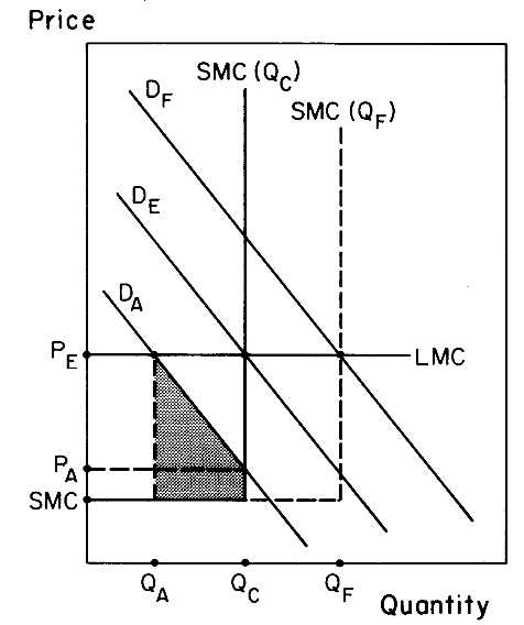
2.1. The future price is likely to be P_K [where D_F = SMC(Q_N .)]. D_A = actual current demand, D_E .: = erroneous earlier forecast of current demand, D_F ,. = forecast of future demand, SMC(Q_C ) = short-run marginal costs with capacity Q_C , SMC(Q_F ) = short-run marginal costs with capacity Q_F , LMC = long-run marginal cost. The hatched area is the short-run loss of using P_E ,: rather than PA as the current price.

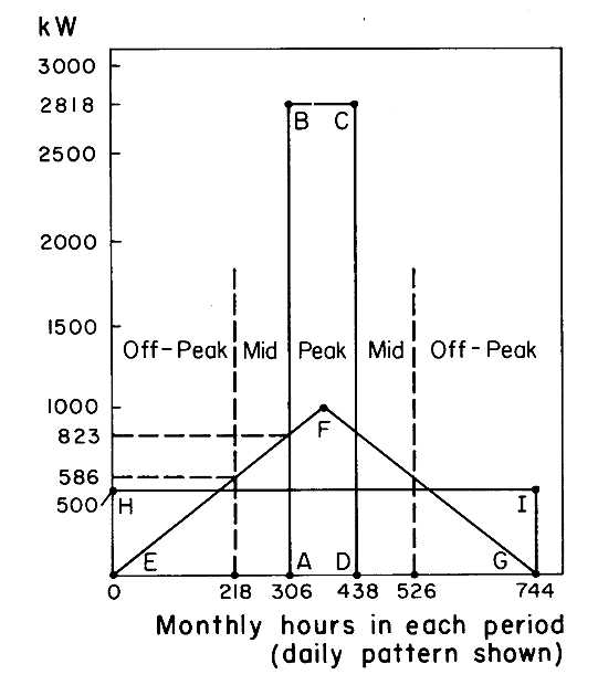
2.2. Patterns of kilowatt demand by time of day.

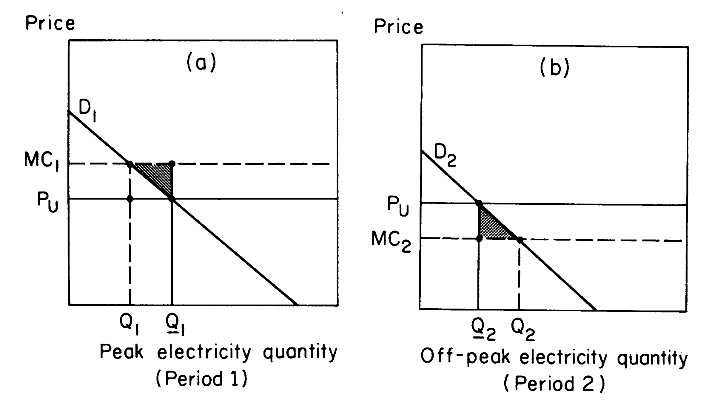
2.3. The efficiency gains from peak-load pricing (shaded):
(a) period 1 (peak), (b) period 2 (off-peak).

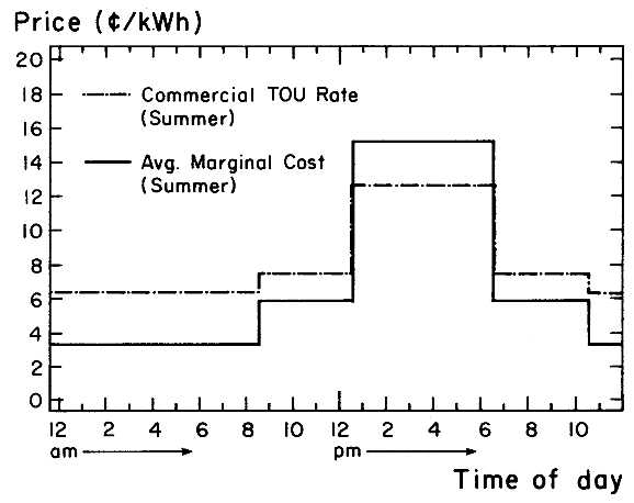
2.4. PG&E summer marginal cost and commercial TOU rates.