8—
CLASSIFICATION, INVENTORY, AND MONITORING OF RIPARIAN SYSTEMS

Evolution and Riparian Systematics^[1]

David E. Brown^[2]

Abstract.—Arizona's perennial streams and important marshlands have been mapped and a wetland classification system developed. To be effective and usable, a resource classification must be systematic, universal, and hierarchical, and must illustrate, or at least recognize, evolutionary relationships. Biogeography is therefore an important factor in the development of the taxonomy for any living (i.e., renewable) resource. Few renewable resources are as alive and dynamic as are our riparian ecosystems.

We have mapped Arizona's perennial streams and important wetlands at 1:1,000,000 (Brown etal . 1977, 1978, 1981). These maps show the potential for maximum riparian ecosystem development—various riparian communities are not illustrated perse . Riparian communities are too dynamic to present the same structure and composition for any length of time; similar communities may also occur along seasonal and even some ephemeral subterranean-fed waterways. This does not mean that riparian vegetation cannot be inventoried and mapped for study purposes and to document change.

We have developed a classification system that includes riparian and other wetland communities as well as upland ecosystems (see Appendix A) (Brown and Lowe 1974a, 1974b; Brown etal . 1977, 1979, 1980). Like the Linnean taxonomic system, this classification system is systematic in approach, universal in application, and hierarchical in arrangement. It is also digitized and therefore computer-compatible. Like other ecosystem classifications, this system uses vegetation, structure, climate, and vegetative components as criteria. However, an important distinction is that it is based on biogeography.

A classification based on this system for use in the Southwest has proven serviceable for classification, delineation, description, and data storage of that region's natural vegetation and biogeography. For examples of its application see Turner and Cochran (1975), Steenbergh and Warren (1977), Patton (1978), Martin (1979), Turner etal . (1980), and Volger (1980).

All classifications of vegetation consider structure (i.e., forests, woodlands, grasslands, etc.); the most successful employ phytogeographic descriptions (i.e., floodplain forest, montane forest, coastal scrub, etc.). Unfortunately, many of these same classifications rely on soil and/or chemical criteria which influence floristics only regionally. Soil-types or soil properties are of little use in describing vegetation on a worldwide or even continental basis. Some systems (e.g. Bailey 1976, 1978) use physiographic approaches that are wholly regional in scope and bear little relationship to biotic parameters. Few systems employ biogeography as it is used by biologists.

Biologists have long been developing systems of biographic realms, provinces, and districts (e.g., see Wallace 1876; Clements and Shelford 1939; Rasmussen 1941; Pitelka 1941; Dice 1943; Goldman and Moore 1945; Dansereau 1957; Darlington 1957; Lowe 1961; Shelford 1963; Walter 1973; Udvardy 1975; Cox etal . 1976; Dasmann 1976; Franklin 1977) to show the distribution of plants and animals. These distributions are the result of evolutionary origin and adaptation. The basic biogeographic unit is the biome (i.e., biotic community). The biome is also the primary component and mappable reality of any biotic classification system that attempts to illustrate evolutionarily significant plant and animal distribution. Distributions which are of evolutionary significance are of great importance to bird watchers, ornithologists, zoogeographers, mammalogists, herpetologists, phytogeographers, taxonomists, and wildlife managers. Biologists will generally not accept classifications and inventories that do not recognize the importance of biomes and biogeography. This is especially true of our riparian and other wetland resources, so valued for their biotic diversity.

[1] Paper presented at the California Riparian Systems Conference. [University of California, Davis, September 17–19, 1981].

[2] David E. Brown is Wildlife Biologist, Arizona Game and Fish Department, Phoenix; and Professor of Wildlife Management, Arizona State University, Tempe, Ariz.

Literature Cited

Bailey, R.G. 1976. Ecoregions of the United States (map, scale 1:7,500,000). USDA Forest Service, Intermountain Region, Ogden, Utah.

Bailey, R.G. 1978. Description of the ecoregions of the United States. USDA Forest Service, Intermountain Region, Ogden, Utah.

Brown, David E., Neil B. Carmony, and Raymond M. Turner. 1977. Inventory of riparian habitats. p. 10–13. In : R.R. Johnson and D.A. Jones (tech. coord.). Importance, preservation and management of riparian habitat: a symposium. [Tuscon, Ariz., July 9, 1977]. USDA Forest Service GTR-RM-43. 217 p. Rocky Mountain Forest and Range Experiment Station, Fort Collins, Colo.

Brown, David E., Neil B. Carmony, and Raymond M. Turner. 1978. Drainage map of Arizona showing perennial streams and some important wetlands. Ariz. Game and Fish Department map.

Brown, David E., Neil B. Carmony, and Raymond M. Turner. 1981. Drainage map of Arizona showing perennial streams and some important wetlands. Ariz. Game and Fish Department map.

Brown, David E., and C.H. Lowe. 1974a. A digitized computer-compatible classification for natural and potential vegetation in the Southwest with particular reference to Arizona. J. Ariz. Acad. Sci. 9, Suppl. 2:1–11.

Brown, David E., and C.H. Lowe. 1974b. The Arizona system for natural and potential vegetation—illustrated summary through the fifth digit for the North American Southwest. J. Ariz. Acad. Sci. 9, Suppl. 3:1–56.

Brown, David E., C.H. Lowe, and C.P. Pase. 1977. A digitized classification system for the natural vegetation of North America with hierarchical summary for world ecosystems. In : A. Marmelstein (ed.). Proceedings of the national symposium on classification, inventory, and analysis of fish and wildlife habitat. [Phoenix, Ariz., Jan. 24–27, 1977]. USDI Fish and Wildlife Service, Office of Biological Science, Washington, D.C.

Brown, David E., C.H. Lowe, and C.P. Pase. 1979. A digitized classification system for the biotic communities of North America, with community (series) and association examples for the Southwest. J. Ariz.-Nev. Acad. of Sci. Suppl. 1:1–16.

Dansereau, P. 1957. Biogeography. Ronald Press. New York, New York.

Darlington, P.J., Jr. 1957. Zoogeography. John Wiley and Sons. New York, New York.

Dansmann, R.F. 1976. Biogeographical provinces. Co-Evolution Q. Fall:32–35.

Dice, L.R. 1943. The biotic provinces of North America. University of Michigan Press. Ann Arbor, Mich.

Franklin, J.F. 1977. The biosphere reserve program in the United States. Science 195: 262–267.

Goldman, E.A., and R.T. Moore. 1945. The biotic provinces of Mexico. J. Mammal. 26:347–360.

Lowe, C.H. 1961. Biotic communities in the sub-Mongollon region of the inland Southwest. J. Ariz. Acad. Sci. 2:40–49.

Martin, P.S. 1979. A survey of potential natural landmarks, biotic themes, of the Mojave-Sonoran Desert Region. Heritage Conservation and Recreation, U.S. Department of the Interior. 358 p.

Patton, D.R. 1978. Runwild-a storage and retrieval system for wildlife habitat information. USDA Forest Service GTR-RM-51:1–8, Rocky Mountain Forest and Range Experiment Station, Fort Collins, Colo.

Pitelka, F.A. 1941. Distribution of birds in relation to major biotic communities. Amer. Midl. Nat. 25:11–137.

Rasmussen, D.I. 1941. Biotic communities of Kaibab Plateau, Arizona. Ecol. Monog. 11:229–275.

Shelford, V.E. 1963. The ecology of North America. University of Illinois Press. Urbana, Ill.

Steenbergh, W.F., and P.L. Warren. 1977. Preliminary ecological investigation of natural community status at Organ Pipe Cactus National Monument. USDI Cooperative National Park Resources Studies Unit, University of Arizona Tech. Rep. No. 3:1–152.

Turner, D.M., and C.L. Cochran, Jr. 1975. Wildlife management unit-37B-pilot planning study. Arizona Game and Fish Department, Fed. Aid Prog. FW-11-R-8, J-1:1–128.

Turner, R.M., L.H. Applegate, P.M. Bergthold, S. Gallizioli, and S.C. Martin. 1980. Range reference areas in Arizona. USDA Forest Service GTR-RM-79:1–34. Rocky Mountain Forest and Range Experiment Station, Fort Collins, Colo.

Udvardy, M.D.F. 1975. A classification of the biogeographical provinces of the world. Internat. Union Conserv. Nature and Natural Resources (IUCN, Morges, Switzerland). Occas. Pap. 18:1–48.

Vogler, L.E. 1980. The Arizona State Museum archaeological site survey system. Ariz. State Mus. Arch. Ser. 128:1–190.

Wallace, A.R. 1876. The geographical distribution of animals, with a study of the relations of living and extinct fauna and as elucidating the past changes of the earth's surface. MacMillan and Co. London, England.

Walter, H. 1973. Vegetation of the earth in relation to climate and the ecophysiological conditions. Translated from the Second German edition by Joy Wieser. English University Press, London; Springer-Verlag, New York, New York.

Appendix A—
A Digitized Classification System for the Biotic Communities of North America, with Community (Series) and Association Examples for the Southwest^[1]

David E. Brown, Arizona Game & Fish Department, Phoenix Charles H. Lowe, University of Arizona, Tucson Charles P. Pase, USDA Forest Service

Introduction

In previous publications on the North American Southwest System we have addressed primarily the North American Southwest region as outlined in Fig. 1 (Brown and Lowe 1973, 1974a,b). Responses to both the classification system and the classification have been favorable in both general interest and use: e.g., Lacey, Ogden, and Foster 1975; Turner and Cochran 1975; Carr 1977; Dick-Peddie and Hubbard 1977; Ellis etal . 1977; Glinski 1977; Hubbard 1977; Pase and Layser 1977; Steenbergh and Warren 1977; Patton 1978; BLM 1978a,b; Turner etal . 1979. In this report we expand the classification nomenclature at digit levels 1–4 to represent the North American continent

The Southwest System is evolutionary in basis and hierarchical in structure. It is a natural biological system rather than primarily a geography-based one in the sense of Dice 1943; Bailey 1978; and others. The resulting classifications are, therefore, natural hierarchies.

Because of the open-ended characteristic of a natural hierarchical system, resulting classification provides for orderly change. The inherent accordion-type flexibility provides for expansion and contraction at all levels. It permits accommodation of new information into the classification—addition, transference, and deletion of both (a) ecological taxa, and (b) quantitative data on ecological parameters concerning taxa, as our knowledge accumulates on either or both. Digit levels 7 to n accommodate the latter and digit levels 1–6 accommodate the former (ecological taxa) on a world-wide basis.

The system's potential is the provision of a truly representative picture for biotic environment. It permits but does not require inclusion of any and all biotic criteria in a given classification—animals as well as plants. Thereby included in the system's uses are the mapping of wildlife habitats and the determination and delineation of natural areas on a local to world-wide basis (Brown, Lowe, and Pase 1977). On a local basis, overlapping soil mapping units can provide "habitat-types" with their implied biotic potential for land use planning purposes.

The digitation of hierarchy makes the system computer-compatible; e.g., a system or subsystem for storing and retrieving biotic resource data within or parallel to an overall management system. The Southwest System is currently in use in the RUNWILD program developed for field unit use on remote terminals by Region 3 of the Rocky Mountain Forest and Range Experiment Station, U.S. Forest Service (Patton 1978). The system and classification is similarly incorporated in the State of Arizona Resources Inventory System  (ARIS). It is currently used by both industry and agencies for biological studies, resource inventories, and procedures for environmental analysis, for example as required by the National Environmental Policy Act.

The system is responsive to scale. The hierarchical sequence permits mapping at any scale, and various levels of the system have been mapped at 1:1,000,000 (1 inch represents ca. 16 miles). 1:500,000, 1:250,000, 1:62,500 (1 inch represents ca. 1 mile), and others. Moreover, the use of hierarchical sequence permits the needed flexibility for mapping those complex communities where more intensive levels are impractical or needlessly time consuming in a given investigation.

The classification has been expanded to include the major biotic communities of North America (Brown, Lowe, and Pase 1977, 1979). To facilitate communication with potential users, we provide, in addition to some structural modification of the original classification, a number of additional definitions and explanations. Our fourth level (biome) examples for North America are representative; they are not intended as either a definitive or final classification. Examples of the use of the system to the fifth (series = community) and sixth (association) levels are given here for those biomes located wholly or partially within the North American Southwest.

Incorporated in the present classification are contributions from approximately one hundred investigators, primarily biogeographers, wildlife biologists, and ecologists, all of which pertain to or are in general use in the Southwest today. Additional references are given in Brown and Lowe 1974a,b, 1977.

A Digitized Hierarchy of the World's Natural Ecosystems

Where:
1,000 = Biogeographic (Continental) Realm
   1,100 = Vegetation
      1,110 = Formation-type
         1,111 = Climatic (Thermal) Zone
            1,111.1 = Regional Formation (Biome)
               1,111.11 = Series (Community of generic dominants)
                  1,111.111 = Association (Community of specific dominants)
                     1,111.1111 = Composition-structure-phase

A number preceeding the comma (e.g., 1 ,000) refers to the world's biogeographic realms (see Table 1). Origin and evolutionary history are recognized as primary in importance in the determination and classification of natural ecosystems. The mapable reality of the world's biogeographic realms is interpretive in part and dependent on criteria used. In those regions where the components of one realm merge gradually with those of another and the assignment of biogeographic origin is difficult, we include such transitional areas (wide ecotones) in both realms. The following seven realms are adapted from Wallace 1876; see also Hesse etal . 1937; Dansereau 1957; Darlington 1957; Walter 1973; I.U.C.N. 1974; DeLaubenfels 1975; Cox et al . 1976:

[1] A contribution of the Arizona Game and Fish Department with (publication funded by Federal Aid Project W-53R). The University of Arizona Department of Ecology and Evolutionary Biology, and the United States Forest Service, Rocky Mountain Forest and Range Experiment Station.

Figure 1.
The Southwest. In delineating a  natural  Southwest region, approximately one half of the area falls in the
Republic of Mexico and one half in the United States; the U.S. states of "Arizona and New Mexico"
constitute less than half of the "American Southwest." Parts or all of the following states are
included: Arizona, Baja California, California, Chihuahua, Coahuila, Colorado, Nevada, New
Mexico, Sonora, Texas, Utah. All of Baja California and its associated islands (not
completely shown) are included in our concept of a natural North American Southwest
region; extreme northern Durango and Sinaloa are also included at Lat. 26º N.

First Level.—The first digit after the comma (e.g., 11 ,00) refers to vegetation, the structural and readily measurable reality of ecosystems. Included are all potential and/or existing plant communities that are presumed to be established naturally under existing climate and the cessation of artificially disruptive (man-caused) influences^[2](Table 1).

All existing and potential natural vegetation (PNV) is classified as belonging to uplands (1,100) or wetlands (1,200) as in Table 1. Cultivated lands are designated 1,300 (cultivated uplands) and 1,400 (cultivated wetlands). The evolutionary distinctions between plants and animals of terrestrial (upland) ecosystems and those of aquatic or hydric (wetland) ecosystems is recognized by this dichotomy (see Ray 1975).

As discussed here, wetlands include those periodically, seasonally or continually submerged ecosystems populated by species and/or life forms different from the immediately adjacent (upland) climax vegetation, and which are dependent on conditions more mesic than provided by the immediate precipitation. Certain ecosystems having both upland and wetland characteristics and components (e.g., riparian forests) could be properly considered as belonging to both divisions. They are treated in this report as wetlands (1,2 00).

Second Level.—The second digit after the comma (e.g. 1,11 0) refers to one of the following recognized ecological formations, which on a worldwide basis are the formation-types (biome-types); see Tables 2 and 3. On continents these are referred to as formations, which are vegetative responses (functions) to integrated environmental factors, most importantly plant-available moisture.

Upland Formations

[2] Our thinking on the complex question of determining climax, successional, and potential vegetation is to consider (and map) ecosystems on the basis of the existing or presumed vegetation of the foreseeable future.

[3] The holistic integrity of a "Tundra" formation is not without question. Treated here, tundra may also be composed of grasslands, scrublands, marshlands (wet tundra), and desertlands in an Arctic-Boreal climatic zone (Billings and Mooney 1968; Billings 1973; and others.

[4] The "savanna" formation (Dansereau 1957; Dyksterhuis 1957; and others) is here recognized (in North America) as an ecotone between woodland and grassland. Those homogeneous areas in which the crowns of trees normally cover less than approximately 15 percent of the ground space are classified as grasslands where grasses are actually or potentially dominant (=savanna grassland). Mosaics of grassland and smaller or larger stands of trees and shrubs are "parklands" and are composed of two or more ecologically distinct plant formations (Walter 1973).

Wetland Formations

Some localized upland and wetland areas are essentially without vegetation or are sparingly populated by simple organisms, e.g., on some dunes, lava flows, playas, sinks, etc. For purposes of classification certain of such areas could be considered as belonging to a nonvegetated formation-type (Tables 2 and 3).

Third Level.—The third digit beyond the comma (e.g., 1,111) refers to one of four world climatic zones (c.f. Walter 1973; Ray 1975; Cox etal . 1976), in which minimum temperature remains a major evolutionary control of and within the zonation and the formation-types (Tables 4 and 5). All four of these broad climatic zones are found in North America and in the "Southwest."

Fourth Level.—The fourth digit beyond the comma (e.g., 1,111.1 ) refers to a subcontinental unit that is a major biotic community (=biome). Biomes are natural communities characterized by a distinctive vegetation physiognamy within a formation; accordingly, the natural geography of biomes is commonly disjunctive. A single biome is not to be confused with a single biotic (biogeographic) province; in distribution, a province is always a continuous (non-disjunctive) biogeographic area that may include several (e.g., five or more) biomes.^[7]

Our nomenclature at the biome (fourth) level incorporates useful geographic terms in the same sense of Weaver and Clements (1938). While such terms are also associated with biotic provinces (as in Fig. 2) we are classifying biomes, not biotic provinces. Biomes are characterized by a distinctive evolutionary history within a formation; thus they tend to be centered in, but are not restricted to particular biogeographic regions or provinces (e.g., see Weaver and Clements 1938; Clements and Shelford 1939; Pitelka 1941, 1943; Dice 1939, 1943; Odum 1945; Allee etal . 1949; Kendeigh 1954, 1961; Dansereau 1957; Shelford 1963; Daubenmire and Daubenmire 1968; Udvardy 1975; Dasmann 1976).

This fourth level and the fifth level (below) have provided the most successful and useful mapping of states, regions, and continents (e.g., in North America, Harshberger 1911; Shreve 1917, 1951; Shantz and Zon 1924; Bruner 1931; Morris 1935; Wieslander 1935; Brand 1936;

[5] Treated here, tundra may also be composed of grasslands, scrublands, marshlands (wet tundra), and desertlands in an Arctic-Boreal climatic zone; see footnote 3.

[6] Strand communities are situated in harsh physical environments that produce their characteristic physiognomy. Accordingly, strandland is treated as the wetland equivalent of desertland. While occurring in the usual sense on beaches and other seacoast habitats, freshwater (or interior) strands also occur in river channels, along lake margins, and below reservoir high water lines.

[7] Originally termed biotic provinces by Lee Dice (1943) who developed this biogeographic concept in North America between 1922 (biotic areas) and 1943 (biotic provinces), they have been referred to variously in recent literature as "biotic provinces" (Dasmann 1972, 1974; IUCN 1973), "biogeograpt' provinces" (Udvardy 1975; Dasmann 1976). "ecoregions" (Bailey 1976, 1978), and "biotic gions" (Franklin 1977).

Nichol 1937; LeSueur 1945; Jensen 1947; Leopold 1950; Castetter 1956; Küchler 1964, 1977; Brown 1973; Franklin and Dyrness 1973; Brown and Lowe 1977). Biomes and biogeographic provinces are also the bases for the biosphere reserve program (MAB) in the United States and elsewhere (IUCN 1974; Franklin 1977).

A partial summary of the biotic communities (biomes) for Nearctic and adjacent Neotropical America is given in Tables 6 and 7.

Fifth Level.—The fifth digit beyond the comma (e.g., 1,111.11 ) refers to the principal plant-animal communities within the biomes, distinguished primarily on taxa that are distinctive climax plant dominants. Daubenmire and Daubenmire (1968) organized their data according to major dominants in climax communities referred to as climax series. "Series," or "cover-types" (sensu Society of American Foresters 1954), or "vegetation-types" (sensu Flores etal . 1971), are each composed of one or more biotic associations characterized by shared climax dominants within the same formation, zone, and biome (Oosting 1950; Lowe 1964; Franklin and Dyrness 1973; Pfister etal . 1977). For example, within Rocky Mountain montane conifer forest (122.3), the Pine Series (122.32) includes all of the Rocky Mountain forest associations in which Pinus ponderosa is a dominant.

Community diversity of tropical and subtropical upland climax dominants is inherently more complex than in boreal and temperate communities. Moreover, some taxa may exhibit polymorphism to the extent that the same species may be dominant—and ecotypically differentiated—in more than a single formation. As an extreme case in southwestern North America, mesquite (Prosopisjuliflora ) may be a dominant life-form in certain desertland, disclimax grassland, scrubland, woodland, and riparian forest communities, and exhibit phenotypic and presumably genotypic population differentiation across the complex gradient. Facultative growth-form is exhibited by dominant plant taxa in both cold and warm climatic zones.

The distribution of some plant dominants also may span more than a single climatic zone, as in Larrea, Prosopis, and the introduced Tamarix. However, important plant and animal associates of these dominant species are usually encountered when passing from one formation or climatic zone to another. When specific and generic dominants are shared by more than one biome, closer investigation may reveal genetic geographic variation within the shared species, as in the chromosome races of creosotebush (Larrea divaricata, Yang and Lowe 1968; Yang 1970).

It is clear that the determination of fifth and sixth (below) level communities in particular will require modification and revision in the classification as field data accumulate. Some of the more widely distributed and commonly recognized series in the Southwest are given in Tables 6 and 7 under the appropriate biome.

Sixth Level.—The sixth digit beyond the comma (e.g., 1,111.111 ) refers to distinctive plant associations, and associes (successional associations), based on the occurrence of particular dominant species more or less local or regional in distribution and generally equivalent to habitat-types as outlined by the Daubenmires (1968), Layser (1974), Pfister et al . (1977), and others. While we give examples for certain communities within southwestern biomes, the enormous numbers of sets precludes presentation here for the treatments given in Tables 6 and 7. Associations may be added at length for regional studies by using a, b, c, sets as is also indicated in the tables in Brown and Lowe (1974a,b).

Seventh Level.—The seventh digit beyond the comma (e.g., 1,111.1111 ) accommodates detailed measurement and assessment of quantitative structure, composition, density and other attributes for dominants, understories, and other associated species. This level and additional ones in the system provide the flexibility required for encompassing data for ecological parameters measured in intensive studies on limited areas (see e.g., Dick-Peddie and Moir 1970).

Figure 2.
Biogeographic provinces of Nearctic and adjacent Neotropical North America (modified
after Dice 1943, and Dasmann 1974), discussed in text under fourth (Biome) digit level.

Literature Cited

ALLEE, W. C., A. E. EMERSON, O. PARK, T. PARK, and K. P. SCHMIDT. 1949. Principles of Animal Ecology. W. B. Saunders Co., Philadelphia.

BAILEY, R. G. 1976. Ecoregions of the United States (map, scale 1:7,500,000). USDA Forest Serv., Intermtn. Region, Ogden, Utah.

__________. 1978. Description of the Ecoregions of the United States. USDA Forest Serv., Intermtn. Region, Ogden, Utah.

BARBOUR, M. G. and J. MAJOR (eds.) 1977. Terrestrial Vegetation of California. John Wiley and Sons, New York.

BILLINGS, W. D. 1973. Tundra grasslands, herblands and shrublands and the role of herbivores. In R. H. Kesel (ed.) Grassland Ecology. Louisiana St. Univ. Press, Baton Rouge.

__________ and H. A. MOONEY. 1968. The ecology of arctic and alpine plants. Biol. Rev. 43:481–529.

BRAND, D. B. 1936. Notes to accompany a vegetation map of northwestern Mexico. Univ. New Mexico, Biol. Ser. 4:5–27.

BROWN, D. E. 1973. The Natural Vegetative Communities of Arizona (map, scale 1:500,000). State of Arizona, Ariz. Resources Information System (ARIS), Phoenix.

__________ and C. H. LOWE. 1973. A proposed classification for natural and potential vegetation in the Southwest with particular reference to Arizona. Ariz. Game and Fish Dept., Fed. Aid Proj. Rep. W-53R-22-WP4-J 1:1–26.

__________ and __________. 1974a. A digitized computer-compatible classification for natural and potential vegetation in the Southwest with particular reference to Arizona. J. Ariz. Acad. Sci. 9, Suppl. 2:1–11.

__________ and __________. 1974b. The Arizona system for natural and potential vegetation—illustrated summary through the fifth digit for the North American Southwest. J. Ariz. Acad. Sci. 9, Suppl. 3:1–56.

__________ and __________. 1977. Biotic communities of the Southwest. USDA Forest Serv., Rocky Mtn. Forest and Range Exp. Stn., Gen. Tech. Rep. RM-41 :map, scale 1:1,000,000.

__________, __________, and C. P. PASE. 1977. A digitized classification system for the natural vegetation of North America with hierarchical summary for world ecosystems. In A. Marmelstein (1979) (ed.) Proc. National Symposium on Classification, Inventory, and Analysis of Fish and Wildlife Habitat, Jan. 24–27, 1977, Phoenix, Arizona. USDI Fish and Wildlife Serv., Off. Biol. Sci., Washington, D.C.

__________,__________, and __________. A Digitized Systematic Classification for Ecosystems with an Illustrated Summary of the Vegetation of North America. USDA Forest Service (in press).

BRUNER, W. E. 1931. The vegetation of Oklahoma. Ecol. Monogr. 1:99–188.

BUREAU OF LAND MANAGEMENT. 1978a. Draft Environmental Statement—Proposed livestock grazing program Cerbat/Black Mountain Planning Units. USDI, BLM Arizona State Office, Phoenix.

__________. 1978b. Upper Gila-San Simon Grazing environmental statement draft. USDI, BLM Arizona State Office, Phoenix.

CARR, J. N. 1977. Arizona Game and Fish Department comprehensive five year plan. Ariz. Game and Fish Dept., Fed. Aid Proj. FW-11-R-9, 1:1–12.

CASTETTER, E. F. 1956. The vegetation of New Mexico. New Mexico Q. 26:257–288.

CLEMENTS, F. E., and V. E. SHELFORD. 1939. Bio-ecology. John Wiley and Sons, New York.

COX, B. C., I. N. HEALY, and P. D. MOORE. 1976. Biogeography, an Ecological and Evolutionary Approach. 2nd ed. Blackwell Science Publ., Oxford.

DANSEREAU, P. 1957. Biogeography. Ronald Press, New York.

DARLINGTON, P. J., JR. 1957. Zoogeography. John Wiley and Sons, New York.

DASMANN, R. R. 1972. Towards a system for classifying natural regions of the world and their representation by national parks and reserves. Biol. Conserv. 4:247–255.

DASMANN, R. F. 1974. See I.U.C.N. 1974.

__________. 1976. Biogeographical provinces. Co-Evolution Q. Fall:32–35.

DAUBENMIRE, R. and J. DAUBENMIRE. 1968. Forest vegetation of eastern Washington and northern Idaho. Wash. Agric. Exp. Stn., Tech. Bull. 60:1–104.

DeLAUBENFELS, D. J. 1975. Mapping the world's vegetation. Syracuse Univ. Press., Geogr. Series 4:1–246.

DICE, L. R. 1922. Biotic areas and ecological habitats as units for the statement of animal and plant distribution. Science 55:335–338.

__________. 1939. The Sonoran Biotic Province. Ecology 20:118–129.

__________. 1943. The Biotic Provinces of North America. Univ. Mich. Press, Ann Arbor.

DICK-PEDDIE, W. A. and W. H. MOIR. 1970. Vegetation of the Organ Mountains, New Mexico. Colorado State Univ. Range Sci. Dept., Sci. Ser. 4:1–28.

__________ and J. P. HUBBARD. 1977. Classification of riparian vegetation. In Importance, Preservation and Management of Riparian Habitat: A Symposium. USDA Forest Serv., Rocky Mtn. Forest and Range Exp. Stn., Gen. Tech. Rep. RM-43:85–90.

DYKSTERHUIS, E. J. 1957. The savannah concept and its use. Ecology 38:435–442.

ELLIS, S. L., C. FALLAT, N. REECE and C. RIORDAN. 1977. Guide to land cover and use classification systems employed by Western governmental agencies. USDI Fish and Wildlife Service.

FLORES MATA, G., J. JIMENEZ LOPEZ, X. MADRIGAL SANCHEZ, F. MONCAYO RUIZ, and F. TAKAKI TAKAKI. 1971. Memoria del mapa de tipos de vegetacion de la Republica Mexicana. Secretaría de Recursos Hidráulicos, Subsecretaría de Planeacion, Direccíon General Estudios, Direccíon de Agrologia, Mexico, D. F. (manual and map, scale 1:2,000,000).

FRANKLIN, J. F. 1977. The biosphere reserve program in the United States. Science 195:262–267.

__________  and C. T. DYRNESS. 1973. Natural Vegetation of Oregon and Washington. USDA Forest Serv., Pac. Northwest Forest and Range Exp. Stn., Gen. Tech. Rep. PNW-8:1-417.

GLINSKI, R. L. 1977. Regeneration and distribution of sycamore and cottonwood trees along Sonoita Creek, Santa Cruz County, Arizona. In Importance, Preservation and Management of Riparian Habitat: A Symposium. USDA Forest Serv., Rocky Mtn. Forest and Range Exper. Stn., Gen. Tech. Rep. RM-43:116–123.

HARSHBERGER, J. W. 1911. Phytogeographic Survey of North America. G. E. Stechert, New York.

HESSE, R., W. C. ALLEE, and K. P. SCHMIDT. 1937. Ecological Animal Geography. John Wiley and Sons, New York.

HUBBARD, J. P. 1977. A biological inventory of the lower Gila River Valley, New Mexico. A report jointly prepared by Bureau of Land Management, Bureau of Reclamation, New Mexico Department of Game and Fish, Soil Conservation Service, U.S. Forest Service.

INTERNATIONAL UNION FOR CONSERVATION OF NATURE AND NATURAL RESOURCES (I.U.C.N.). 1973. A working system for classification of world vegetation. IUCN, Morges, Switzerland, Occas. Pap. 5:1–21.

__________. 1974. Biotic provinces of the world—further development of a system for defining and classifying natural regions for purposes of conservation. IUCN, Morges, Switzerland, Occas. Pap. 9:1–57.

JENSEN, H. A. 1947. A system for classifying vegetation in California. Calif. Fish and Game 33:199–266.

KENDEIGH, S. C. 1954. History and evolution of various concepts of plant and animal communities in North America. Ecology 35:152–171.

__________. 1961. Animal Ecology. Prentice-Hall, Englewood Cliffs, New Jersey.

KUCHLER, A. W. 1964. The potential natural vegetation of the conterminous United States. Amer. Geog. Soc., Spec. Publ. 36:1–116; map, scale 1:3,168,000.

__________. 1977. Natural vegetation of California (map, scale 1:1,000,000). In M. G. Barbour and J. Major (eds.) Terrestrial Vegetation of California. John Wiley and Sons, New York.

LACEY, J. R., P. R. OGDEN and K. E. FOSTER. 1975. Southern Arizona riparian habitat: spatial distribution and analysis. Univ. Arizona, Off. Arid Lands Studies Bull. 8:1–148.

LAYSER, E. F. 1974. Vegetative classification: its application to forestry in Northern Rocky Mountains. J. For. 72:354–357.

LEOPOLD, A. S. 1950. Vegetation zones of Mexico. Ecology 31:507–518.

LeSUEUR, H. 1945. Ecology of the vegetation of Chihuahua, Mexico, north of parallel twenty eight. Univ. Texas Publ. 452:1–92.

LOWE, C. H. 1961. Biotic communities in the sub-Mogollon region of the inland Southwest. J. Ariz. Acad. Sci. 2:40–49.

__________. 1964. Arizona's Natural Environment; Landscapes and Habitats. Univ. Ariz. Press, Tucson.

MORRIS, M. 1935. Natural Vegetation of Colorado (map). In R. E. Gregg (1963), The Ants of Colorado. Univ. Colo. Press, Boulder.

NICHOL, A. A. 1937. The natural vegetation of Arizona. Univ. Ariz. Agric. Exp. Stn., Tech. Bull. 68:181–222, with map.

ODUM, E. P. 1945. The concept of the biome as applied to the distribution of North American birds. Wilson Bull. 57:191–201.

OOSTING, H. J. 1950. The Study of Plant Communities. 2nd ed. W. H. Freeman and Co., San Francisco.

PASE, C. P. and E. F. LAYSER. 1977. Classification of riparian habitat in the Southwest. In Importance, Preservation and Management of Riparian Habitat: A Symposium. USDA Forest Serv., Rocky Mtn. Forest and Range Exper. Stn. Gen. Tech. Rep. RM-43:5–9.

PATTON, D. R. 1978. Runwild—a storage and retrieval system for wildlife habitat information. USDA Forest Serv., Rocky Mtn. Forest and Range Exper. Stn., Gen. Tech. Rep. RM-51:1–8.

PFISTER, R. D., B. L. KOVALCHIK, S. F. ARNO, and R. C. PRESBY. 1977. Forest habitat types of Montana. USDA Forest Serv., Intermtn. Forest and Range Exp. Stn., Gen. Tech. Rep. INT-34:1–174.

PITELKA, F. A. 1941. Distribution of birds in relation to major biotic communities. Amer. Midl. Nat. 25:11–137.

__________. 1943. Review of Dice's "Biotic Provinces of North America." Condor 45:203–204.

RAY, G. C. 1975. A preliminary classification of coastal and marine environments. Internat. Union Conserv. Nature and Natural Resources (IUCN, Morges, Switzerland), Occas. Pap. 14:1–26.

SHANTZ, H. L. and R. ZON. 1924. Natural Vegetation. USDA Atlas of Amer. Agric. Plt. 1, Sec. E (map). Washington, D.C.

SHELFORD, V. E. 1963. The Ecology of North America. Univ. III. Press, Urbana.

SHREVE, F. 1917. A map of the vegetation of the United States. Geogr. Rev. 3:119–125.

__________. 1951. Vegetation and Flora of the Sonoran desert. Vol. 1. Vegetation. Carnegie Inst. Wash. Publ. 591:1–192.

SOCIETY OF AMERICAN FORESTERS. 1954. Forest cover types of North America (exclusive of Mexico). Soc. Amer. Foresters, Washington, D.C.

STEENBERGH, W. F. and P. L. WARREN. 1977. Preliminary ecological investigation of natural community status at Organ Pipe Cactus National Monument. USDI Cooperative National Park

       Resources Studies Unit, Univ. Ariz., Tech. Rep. No. 3:1–152.

TURNER, D. M. and C. L. COCHRAN, JR. 1975. Wildlife management unit—37B—pilot planning study. Ariz. Game and Fish Dept., Fed. Aid Prog. FW-11-R-8, J-1:1–128.

TURNER, R. M., L. H. APPLEGATE, P. M. BERGTHOLD, S. GALLIZIOLI, and S. C. MARTIN. Range reference areas in Arizona. USDA Forest Serv., Rocky Mtn. Forest and Range Exper. Stn., Gen. Tech. Rep. (in press).

UDVARDY, M.D.F. 1975. A classification of the biogeographical provinces of the world. Internat. Union Conserv. Nature and Natural Resources (IUCN, Morges, Switzerland), Occas. Pap. 18:1–48.

WALLACE, A. R. 1876. The Geographical Distribution of Animals, with a Study of the Relations of Living and Extinct Faunas and as Elucidating the Past Changes of the Earth's Surface. MacMillan and Co., London.

WALTER, H. 1973. Vegetation of the earth in relation to climate and the ecophysiological conditions. Translated from the 2nd German ed. by Joy Wieser. English Univ. Press, London; Springer-Verlag, New York.

WEAVER, J. E. and F. E. CLEMENTS. 1938. Plant ecology. 2nd ed. McGraw-Hill, New York.

WIESLANDER, A. E. 1935. A vegetation map of California. Madroño 3:140–144.

YANG, T. W. 1970. Major chromosome races of Larrea divaricata in North America. J. Ariz. Acad. Sci. 6:41–45.

__________ and C. H. LOWE. 1968. Chromosome variation in ecotypes of Larrea divaricata in the North American Desert. Madroño 19:161–163.

The Central Valley Riparian Mapping Project^[1]

Charles W. Nelson and James R. Nelson^[2]

Abstract.—The Central Valley Riparian Mapping Project was initiated in 1978 by the California Department of Fish and Game. Maps showing the occurrence of riparian vegetation on the depositional flatland or floor of the Central Valley were compiled from existing aerial photographs (35mm. color slides and high altitude, false-color infrared U-2). Special techniques devised to map from 35mm. color slides are described. Vegetation-types were divided into six riparian categories, two subcategories, and two nonriparian categories. Modifying characters were used to indicate unusual circumstances under which riparian vegetation occurred. These maps provide a record of this diminishing resource on the floor of the Central Valley as it appeared in 1976. This data base will permit the documentation of changes in this important riparian resource in the future.

Introduction

Project Background

The Central Valley Riparian Mapping Project (CVRMP) was the first attempt by the State of California to map, quantify, and monitor the distribution of riparian resources in the Central Valley. The distribution of riparian vegetation has been described by previous investigators using literature searches, early soil surveys, and personal communications (Conrad etal . 1977; McGill 1975; Roberts etal . 1977; Thompson 1961). Detailed mapping of riparian vegetation on the Sacramento River was recently completed by the California Department of Water Resources (DWR) (1978) and contributed significantly to the information on that riparian system. Work by the USDI Fish and Wildlife Service (FWS) (Cowardin etal . 1977) will provide a complete inventory of riparian vegetation in the Central Valley, but at a smaller scale. The CVRMP provided large-scale maps which record the distribution of riparian vegetation and provide a tool for quantifying the amount of this resource remaining in the Central Valley.

Legislation enacted in 1978 (AB 3147, Fazio) appropriated funding to the Department of Fish and Game (DFG) for a study of the riparian resource of California's Central Valley up to the upper edge of the digger pine/blue oak zone (Küchler 1977)—approximately 760-m. (2,500-ft.) elevational level—and the South Lahontan and Colorado Basins of the California Desert. This legislation was intended as a first step toward acquiring the data needed to properly care for this important and diminished resource.

The CVRMP was an element of the DFG's overall riparian study program and was designed to contribute to development of study recommendations for protection of the resource. In addition, the maps provide a record of the resource as it existed in 1976 (the average date of the aerial photographs). From this data base it will be possible to determine change in the riparian resource in the years to come. The maps can also be used to determine and analyze potential impacts of development upon the resource on a day-to-day basis.

The CVRMP was carried out by two mapping teams comprised of graduate and undergraduate students from California State University, Chico, and California State University, Fresno. While other mapping projects have mapped portions of the Valley's riparian resource, this is the only study that provides complete coverage of the entire Valley floor.

Project Objectives and Scope

The CVRMP was intended to provide a baseline assessment of existing riparian vegetation-types through their categorization and mapping. This study documented the extent and distribution of this resource and provided a basis for quantifying existing riparian vegetation (see Katibah, Nedeff, and Dummer 1981). The results of the

[1] Paper presented at the California Riparian Systems Conference. [University of California, Davis, September 17–19, 1981].

[2] Charles W. Nelson is Cartographic Technician/Lecturer in Geography at California State University, Chico. James R. Nelson is a Botanist with the California Energy Commission, Sacramento.

study have been incorporated into the DFG's fish and wildlife planning effort and are being used to direct riparian studies as well as preservation and restoration programs.

Methods

Aerial photos depicting the Central Valley depositional flatland were used to produce maps of riparian vegetation categories and their spatial distribution. Methods were devised which allowed use of existing aerial photography in an accurate and rapid fashion at the lowest possible cost. A technique was devised to expedite the mapping task using available 35mm. photos. Project team members were trained in the recognition, interpretation, and mapping of riparian vegetation categories.

Imagery

Aerial photography served as the data base for the mapping process. Positive transparencies (35mm. color slides) taken by the DWR over a five-year period (average date 1976) were used as the primary information source for the project. These photos were taken at low altitude (ca. 1,525 m. (5,000 ft.)) and provided coverage for most of the study area. The large scale of this true color (Kodachrome) imagery made interpretation of vegetation-types relatively simple. The 35mm. format was easy to handle during the information transfer process using techniques described below.

For those areas not covered by DWR photography, high altitude, U-2, false-color infrared photography was used. Further coverage was provided by standard panchromatic (black-and-white) 9 × 9-in. photographs.

Interpretation

Interpretation of vegetation categories from aerial photographs was accomplished through careful evaluation of standard image characteristics (i.e., color, pattern, shape, association, size, shadow, and topographic location). A detailed description of the vegetation categorization appears below.

An initial field reconnaissance was conducted to familiarize all team members with the riparian vegetation categories. Discussions were held periodically during the mapping phase to ensure the correct interpretation of unusual photo-signatures and check the accuracy of completed maps. This routine procedure kept all mappers aware of various interpretive and cartographic problems and assured greater accuracy and consistency in the mapping effort. Ground-truth checks were conducted on most maps to further ensure map accuracy.

Data Transfer

The mapping of vegetation over large areas required the development of a system that would allow quick, accurate scale adjustment and adequate illumination of the image onto the base map. For this purpose, a transfer system was devised for the DWR 35mm. color slides.

Information from the 35mm. slides was traced onto mylar or blueline sheet overlays of 1:24,000 USDI Geological Survey (GS) quadrangle maps (quads) through the use of a system which projected the photo-image to the bottom of the map through a glass table. Figure 1 is a schematic diagram of this system. A Kodak Ektographic, high light-intensity slide projector (Model AF-2) with a 3-in. (f:3.5) close-up lens, was used to project the slides. The image was reflected up through the glass tabletop by means of a mirror which was mounted at a 45° angle. Slides were reversed when placed in the projector to allow for the reversal of the reflected image. Scale was adjusted either by moving the mirror toward or away from the projector (major-scale adjustments) or through the use of the projector's focus mechanism (minor-scale adjustments).

Figure 1.
Schematic of the data-transfer system. The image can
be projected at the same scale as the base map,
making transfer work accurate and efficient.

Cartographic Representation

Riparian vegetation categories were represented by polygons outlining each vegetation area. Each vegetation category polygon was labelled with a letter or letter/number code. Where vegetation strips were too narrow to outline (such as along a narrow stream or canal), the vegetation was indicated by a single solid line. Letter codes were placed within the polygon boundaries when space permitted. Where space was limited, they were placed outside, with an arrow drawn to the center of the area. Where the vegetation was indicated by a single line, an arrow was drawn from the category symbol to that line. Where more than one vegetation category occurred on a narrow (single-line) strip, a short perpendicular line indicated the boundary. When a single line intercepted a polygon or another single line, a label was placed on each line segment. Figure 2 is an example of the riparian vegetation map product.

Figure 2.
A sample of the riparian vegetation
map product. Scale = 1:24,000.

Mapping Criteria

The following criteria were used as the basis for mapping.

1) Areas with native or "wild" (nonagricultural) riparian vegetation which could be outlined were always mapped.

2) All continuous natural streamcourses associated wholly or in part with riparian vegetation were mapped. Where a natural stream had discontinuous riparian vegetation sections which were separated by short (e.g., 3.2-km. (2-mi.)) sections of vegetation-types not normally mapped, the entire streamcourse was shown.

3) Canals, discontinuous streams, or wet areas which appeared (from the imagery) to be dependent upon an artificial water source and devoid of woody riparian vegetation were not mapped.

4) Agricultural and urban areas were mapped only when they appeared as islands surrounded by riparian vegetation.

Mapping Category System

The major category system used in the CVRMP was based on structural differences (physiognomy) of vegetation units which could be readily discerned from aerial photography. Vegetation units were divided into six riparian or riparian-associated categories, two subcategories (for minor types occurring as part of major categories), and two nonriparian categories (used where nonriparian lands were surrounded by riparian vegetation). In addition, three modifying characters were used to indicate special circumstances under which riparian vegetation occurs. A "hybrid" system was devised to describe those areas which appear to be a mixture of more than one riparian vegetation category. In such cases, the codes of the two most predominant vegetation categories were indicated.

Riparian Mapping Categories

R1—Large Woody Vegetation

Large woody vegetation refers to the older, well-established riparian forests which are represented by tall (over 12 m.) woody vegetation. In the Central Valley bottomlands these areas are usually dominated by Fremont cottonwood (Populus fremontii ), black walnut (Juglans hindsii ), western sycamore (Platanusracemosa ), Oregon ash (Fraxinuslatifolia ), and willow (Salix gooddingii var. gooddingii and other spp.). Accompanying these species is usually a dense understory of shrubs and vines; wild grape (Vitiscalifornica ), blackberry (Rubus spp.), and mugwort (Artemisia douglassiana ) are a few of these species. This vegetation category may cover large areas along broad undisturbed floodplains or very narrow (sometimes discontinuous) strips where human land-use practices have encroached upon the "wild" vegetation.

The R1 category may be discerned in true color aerial photography on the basis of distinct bright green color or mottled color combinations, the evident pattern of tree crowns, relative topographic location, and occasionally by the occurrence of tree shadows. The color of the R1 category is typically much lighter (at times almost yellow-green) than the R1v category (the only other tall-tree category). R1 often shows color or tonal mottling which results from the occurrence of numerous tree and shrub species. The crowns of individual large trees are usually evident when surrounded by different species. However, a dense even stand of large trees (usually tall cottonwoods) may appear homogeneous throughout; in such cases individual tree crowns are less discernible. However, the occurrence of long shadows or a comparison with associated vegetation usually is adequate to accurately identify the signature as R1.

R1v—Valley Oak Woodland

This subcategory of large woody vegetation (R1) refers to the Valley Oak woodland plant

community. These are mature stands of well-spaced valley oak (Quercuslobata ) without a well-developed woody understory. Valley grassland species dominate the areas between trees. This vegetation category is generally associated with high terrace portions of lower elevation Central Valley rivers.

Valley oak woodland may occur adjacent to other vegetation categories near streams or as discontinuous isolated patches away from streamcourses. Before extensive land clearing, these isolated patches would have been part of larger woodlands associated with the other riparian vegetation categories. R1v can usually be discerned from R1 and R2 categories (large and low woody vegetation, respectively) on the basis of its dark green color. In addition, rounded, well-separated crowns often can be identified in older stands. As valley oaks are large, stately trees, shadows are also a good indicator.

R2—Low Woody Vegetation

This category represents an early successional stage of riparian forest development. Trees are younger, shorter (up to 12 m.), and may occur with shrub species. Willows and young cottonwoods usually dominate, although brush species occur in some areas.

Interpretation characteristics include nearly consistent coloration, an even photographic texture, and association with other vegetation categories. Low woody vegetation is generally light-green or gray-green in color. It usually appears as a consistently dense, closely spaced stand, although spottiness may occur. As an early successional type, this vegetation category can be expected to occur along sandbars, receding oxbow lakes and sloughs, and in disturbed areas such as canals and levees. It sometimes appears as an intermediate between open water (or sandbars) and the taller riparian forests. Also, it may occur alone, expecially along smaller streams in the lower foothills.

R3—Herbaceous Vegetation (Valley Grasslands)

Valley grasslands includes low (usually less than 1 m.), introduced and native herbaceous species which are mostly annual, although there are some perennial species. Occurrence may be natural (e.g., Valley Grassland plant community or perennially green herbaceous areas along streams) or the result of severe disturbance (constituting an early successional stage).

Two types of riparian-associated herbaceous vegetation were found in the Central Valley. Valley grasslands are treeless, low in stature, and brown during the summer months. In agricultural areas of the Central Valley they are almost exclusively located within a riparian corridor (i.e., uncultivated streamside lands) and may be surrounded by other kinds of riparian vegetation.

The other type of herbaceous riparian vegetation usually occurs along perennial streamcourses on Valley rangeland. It is low in stature, with little or no woody vegetation in evidence, but is green during the summer months, in contrast to the brown of the surrounding rangelands.

R3p—Perennial Seeps

This is a special subcategory of R3 referring to spring areas that are perennially green with herbaceous vegetation. This subcategory is not used for perennially green areas along streams and is differentiated by its patchiness and separation from streamside R3. Artificial seeps, such as those associated with irrigation canals, wells, or windmills, were not included in this subcategory.

M—Marsh

The marsh vegetation category includes intermittent or perennially wet areas with emergent herbaceous vegetation. These areas are characterized by dense stands of tall grass-like plants such as tules (Scirpus spp.), cattail (Typha spp.), sedges (Carex spp.), and rushes (Juncus spp.). These plants are found in, and sometimes interspersed with, continuously moist areas of mud, or standing or sluggishly-moving shallow water. Marsh areas are commonly associated with rivers, streams, lakes, canals, or depressions (sinks).

Marshes can be distinguished on aerial photographs on the basis of color, pattern, location, and association with other vegetation categories. On the photos, marsh appears as a mixed lightor dark-green color. The arrangement of marsh species varies from highly mixed stands (seen as mottled shades of green on the aerial photographs) to homogeneous bands around open pools (which appear as concentric rings around water areas). Marshes are usually found adjacent to or along canals, streams, sinks, and sloughs. They are often found adjacent to willows and herbaceous vegetation. Marsh occurring within channelized streams is often indiscernible. Where marsh occurs with taller mature forests, it is difficult to recognize except in instances where it covers very large areas. Since marsh vegetation was mapped only when it was found among or adjacent to other riparian vegetation categories, not all of the Central Valley marshland was mapped.

S—Sandbars and Gravelbars

Areas of sand and gravel or exposed rock are included in this mapping category. Vegetation is usually limited to very low willows, cottonwoods, and intermittent herbaceous growth undiscernible from the aerial photographs. Usually sandbars and gravelbars occur adjacent to a stream channel. Photographic signatures include white, gray, and brown colors.

W—Open Water

The open water classification includes standing or moving open waterways which are significantly free of vegetation. Sometimes these areas were difficult to interpret (especially where standing water was surrounded by tall, overhanging vegetation), as often this water displays a dull green color, flatness, and a very smooth, even texture, with occasional reflections evident on the aerial photographs. In other situations (particularly with moving water) the color may be darker. Where white areas occur, riffles or rapids may be present. Open water is usually apparent in stream and river channels. In areas where water cannot be seen on the photographs, even though it may be present, it was not mapped. Only water associated with riparian vegetation was mapped. For example, most manmade canals and reservoirs in the Central Valley were not mapped when devoid of significant riparian vegetation.

A—Agriculture

Agricultural lands partially or completely surrounded by riparian vegetation are included in this category. All cultivated and recently cleared lands are included. Agricultural areas which are adjacent to, but not surrounded by, riparian vegetation were not mapped.

U—Urban

The urban category includes those built-up areas which are completely surrounded by riparian vegetation. In practice, this mapping unit was seldom used. Any land cleared of its natural vegetation and put to industrial, commercial, or residential use would fall into this category.

Modifiers

The following modifying codes were used to signify special circumstances under which riparian vegetation might be found.

c—Channelized

This modifier was used where riparian vegetation exists along a watercourse which appears to have been modified by human activity to the point that natural stream contours are no longer visible.

d—Disturbed

Areas of severe man-caused soil disturbance were included within this modifier. Dredger tailings and gravel mining operations are the most common examples. Numerous ponds are found in some of these areas. Ridges of unvegetated gray rock occurring on the more recent sites indicate dredger tailings. At older locations, these ridges may be vegetated with a thin covering of herbaceous growth. Linear strips of R1 or R2 frequently occur between ridges. Most dredger tailings are ilustrated on GS 7.5 minute quads, confirming suspected identifications. Gravel mining may be identified by the presence of vegetated or unvegetated ponds or pits, especially if they have an unnatural shape.

i—Intermittent

Intermittent was used to designate spottiness or nonconsistent occurrence of a given vegetation category. When used with a single code symbol, or both code symbols of a hybrid notation, the interspaced areas should be interpreted as either S, W, and/or R3.

Category Hybrids

Where any area of vegetation could not be classified clearly as one of the major categories or subcategories, a "hybrid" of two codes was used. This was intended to allow for the most accurate representation of areas which have a mix of vegetation categories occurring in spaces too small to map individually. The hybrid system identified only the two most common vegetation categories, even though other types may be present.

The hybrid code itself consists of codes from the two most prominent categories, separated by a slash. The first of the codes represents the category which, on the basis of general appearance, seems to cover the greatest area. The other portion of the hybrid code covers the second largest portion of the outlined area. For example, an area of 45% R1, 35% R2, and 20% of any other vegetation was labeled R1/R2.

Where modifiers were needed, they were placed at the end of the hybrid code (e.g., R1/R2c indicates a canal which is lined with mixed R1 and R2 vegetation). Where a modifier is used, it refers to both portions of the hybrid symbol (e.g., R1/R2ic would indicate a channelized stream lined with intermittent, mixed woody vegetation).

Table 1 presents a summary of the vegetation codes, their descriptions, and the characteristics by which they were identified on the aerial photographs.

Literature Cited

Conrad, S.A., R.L. MacDonald, and R.F. Holland. 1977. Riparian vegetation and flora of the Sacramento Valley. p. 47–55. In : A. Sands (ed.). Riparian forests of California: their ecology and conservation. Institute of Ecology Pub. No. 15. 121 p. University of California, Davis.

Cowardin, L.M., V. Carter, F.C. Golet, and E.T. LaRae. 1977. Classification of wetlands and deep-water habitats of the United States (an operational draft). USDI Fish and Wildlife Service. Unpublished manuscript.

California Department of Water Resources. 1978. Sacramento River Environmental Atlas. California Resources Agency, Sacramento.

Katibah, E.F., N.E. Nedeff, and K.J. Dummer. 1983. Summary of riparian vegetation areal and linear extent measurements from the Central Valley Riparian Mapping Project. In : R.E. Warner and K.M. Hendrix (ed.). California Riparian Systems. [University of California, Davis, September 17–19, 1981]. University of California Press, Berkeley.

Küchler, A.W. 1977. Map of the natural vegetation of California. 1:1,000,000 + 31 p. A.W. Küchler. Department of Geography, University of Kansas, Lawrence.

McGill, R. 1975. Land use changes in the Sacramento River riparian zone, Redding to Colusa. 23 p. Resources Agency, Department of Water Resources, Sacramento, Calif.

Roberts, W.G., J.G. Howe, and J. Major. 1977. A survey of riparian forest flora and fauna in California. p. 3–19. In : A. Sands (ed.). Riparian forests of California: their ecology and conservation. Institute of Ecology Pub. No. 15. 121 p. University of California, Davis.

Thompson, K. 1961. Riparian forests of the Sacramento Valley, California. Annals of the Association of American Geographers 51:294–315.

Current Condition of Riparian Resources in the Central Valley of California^[1]

Edwin F. Katibah, Kevin J. Dummer, and Nicole E. Nedeff^[2]

Abstract.—The riparian resources in California's Central Valley have been greatly reduced and altered in the last 150 years. This paper describes the current condition of the remaining riparian resources in the Central Valley as evaluated with the aid of low-altitude aerial photography. A discussion of several factors influencing riparian resources—grazing, stream channelization, intra-zone and adjacent land uses—is presented. Based on these influences, a qualitative evaluation of the current condition of the remaining riparian resources in the Central Valley is derived.

Introduction

California is a state of vast area and numerous environments, many of which are unique. Riparian vegetation was never a large resource from an areal standpoint, and yet it is a unique environment within the Central Valley, supporting a great variety of plant and animal life.

Most of the riparian vegetation formerly found in the Central Valley is gone today, a casualty of the great and rapid development of the valley. The small amount of riparian vegetation remaining takes on added significance when compared to the vast pristine forests of 150 years ago.

In the mid-1970s, the decline in the areal extent and quality of riparian vegetation was recognized by private conservation organizations. These organizations prompted the California Legislature to enact AB 3147 (Fazio) in August, 1978. This bill funded investigations into the current state of riparian vegetation and helped provide guidelines for the protection and preservation of this resource. The California Department of Fish and Game (DFG), through its Planning Branch, managed the riparian appropriations.

In 1980 the DFG contracted with the Remote Sensing Research Program, Department of Forestry and Resource Management, University of California, Berkeley, to investigate the condition of the riparian vegetation resource found in the Central Valley and adjacent foothills. The tremendous size of the area to be surveyed precluded conventional ground survey techniques from being the primary data source. The use of an aerial photography-aided approach allowed a substantial amount of data to be gathered with minimal expenditures of time and money.

Methodology

The project study area comprised the Central Valley of California, including portions of the surrounding foothills, to the approximate upper edge of the blue oak/digger pine zone (Küchler 1977) (fig. 1). It included all or part of 33 counties and covered 825,540 ha. (20,390,750 ac.).

Sample System Design

The sample system used for this study was comprised of two elements: 1) study area stratification; and 2) sample site allocation within study area strata.

Study Area Stratification

The objective of stratification, as used here, was to reduce the variability of the data collected for resource evaluation. In the case of riparian vegetation, stratification was used

[1] Paper presented at the California Riparian Systems Conference. [University of California, Davis, September 17–19, 1981].

[2] Edwin F. Katibah is Associate Specialist and Kevin J. Dummer is Staff Research Associate, both are with the Remote Sensing Research Program, Department of Forestry and Resource Management, University of California, Berkeley. Nicole E. Nedeff is a Graduate Student, Department of Geography, University of California, Berkeley and is affiliated with the Remote Sensing Research Program.

Figure l.
Central Valley study area.

to segregate the resource into zones (or strata) in which the relationships between samples of vegetation could be meaningfully compared for determining the basic condition of the resource. In order to accomplish this, the study area was stratified by major geo-physical differences, major land uses, and ancillary data pertinent to this investigation.

The geo-physical stratification divided the study area into seven distinct strata:

North Valley Depositional Flatland
North Valley Coastal Foothills
North Valley Sierran Foothills
North Valley Sutter Buttes
South Valley Depositional Flatland
South Valley Coastal Foothills
South Valley Sierran Foothills

The strata were developed from a 1:750,000-scale map of California geology published by the California Division of Mines and Geology. The locations of the geo-physical strata within the study area are shown in figure 2.

Figure 2.
Location of the major geo-physical
strata within the study area.

The land-use stratification recognized three major land-use practices. These three strata—agricultural land use (generally irrigated), dryland agricultural land-use (non-irrigated), and non-agricultural land-use (rangeland, wildland, urban, etc.)—were deemed important to the analysis of the riparian vegetation resource. The land-use strata were derived from the manual interpretation of 1:1,000,000 Landsat color composite imagery of the central California area (Wall etal . 1980).

Finally, a set of riparian vegetation maps (Central Valley Riparian Mapping Project 1979) was used to designate two more strata within the study area: areas mapped for riparian vegetation and areas not mapped for riparian vegetation. Of the 649 1:24,000 USDI Geological Survey (GS) quadrangle maps (quads) needed to cover the study area, 388 were mapped for riparian vegetation.

The final product of these three distinct stratifications yielded 39 unique combinations of geo-physical units, land use, and riparian map-

ping status. These strata were called primary strata and were the basis for the sample allocation strategy. Figures 3 and 4 show the distribution of two primary strata in the study area: Depositional Flatland; Agriculture, Mapped; and Depositional Flatland, Non-agriculture, Mapped.

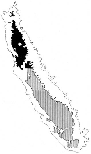
Figure 3.
Distribution of the Depositional Flatland, Agriculture,
Mapped primary stratum in the study area. The north and
south valley portions of this stratum are also identified.
Darker shading indicates the north valley stratum.

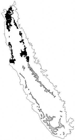
Figure 4.
Distribution of the Depositional Flatland, Non-agriculture,
Mapped primary stratum in the study area. The north and
south valley portions of this stratum are also identified.
Darker shading indicates the north valley stratum.

Sample-Site Allocation

In order to gather information in a systematic and meaningful way, a sampling strategy was developed. By evaluating the variables that dictated the number of samples that could be taken (aircraft availability, project time, available funds, etc.) it was determined that 188 sample sites could be overflown and photographed.

Next, the 188 potential sample-sites were distributed among the primary strata. First, equal sampling weights were assigned to the north and south valley strata, allocating 94 samples to each. Secondly, the individual area for each primary stratum was determined. Each area was converted to a percentage of the total area for the north or south valley strata, as appropriate. The individual primary strata area percentages were then multiplied by the total number of sample sites possible (94 in each case).

Actual location of sample-sites within primary strata was done one of two ways, depending on whether or not the area had been mapped for riparian vegetation. For primary strata defined, in part, by the occurence of riparian vegetation

mapping, samples were allocated as follows. All 1:24,000 quads covering a particular primary stratum were indexed and recorded. In each primary stratum, the set of GS quads was randomly ordered. The sample size value for each primary stratum dictated the number of GS quads selected from the randomly organized map set. Next, a 600-point grid was fitted to each map sheet (corresponding maps with riparian vegetation indicated were used in place of the GS quads). A grid point was randomly selected on each map sheet. If no riparian vegetation occurred under the point selected, the nearest riparian vegetation on the map sheet was selected. This process was continued until all sample sites were located for the primary strata occurring in previously mapped (for riparian vegetation) strata.

For those primary strata not having a previously mapped component, a different sample-site location system had to be employed. The 600-point grid was again fitted to a GS quad from a randomly ordered set, as before. This time the identifiable stream nearest to the randomly selected point was found. This stream was then located on 1:120,000 9- × 9-in., color infrared transparencies (flown by NASA-Ames Research Center in support of the University of California and DWR Irrigated Lands Project). Riparian vegetation and accessibility were quickly evaluated before final selection of the actual sample-sites. Only in a few cases (e.g., where streams were virtually inaccessible), was a potential sample-site rejected. Figure 5 shows the distribution of sample-sites in the study area.

With the sample-site selection completed, a full set of GS quads was compiled with the exact sample sites annotated on each appropriate map. Next, all sample-sites were located and plotted on county road maps. Based on the overall location of the sample-sites with relation to each other, flight plans were developed to facilitate the orderly photographing of each.

Figure 5.
Distribution of sample-sites in the study area.

Aerial Photography

Camera System

The photographic system was comprised of cameras, camera mount, and supporting equipment. Two Hasselblad ELM (motorized) cameras were used for all photography. Both cameras were fitted with magazines capable of holding 15 ft. of 70mm. aerial film. Different lenses were used on the two cameras: a 100mm. f3.5 Zeiss Planar, fitted with an ultraviolet filter for natural color photography, and a 50mm. f4 Zeiss Distagon, fitted with a red (No. 25) filter for black-and-white infrared photography.

The camera mount was designed to hold the two cameras side-by-side in a vertical position. The mount was fitted with an auxiliary viewfinder etched with markings showing the approximate photo center and calibrated to give the desired overlap necessary for stereo photography. The mount was designed to rotate horizontally and to tip, allowing the photographer to correct for aircraft crab and tilt.

Both cameras were fitted with an intervelometer. The intervelometer was connected to a command unit which allowed the cameras to be triggered simultaneously. The time setting on the intervelometer was calibrated by comparing the firing rate of the cameras with the ground-glass image as seen in the camera mount viewfinder.

Film

Two film types were used for this study: 70mm. Kodak Ektachrome MS, Type 2448; and 70mm. Kodak Infrared Aerographic, Type 2424. The Ektachrome MS was intended to provide the main product used in the photo-interpretation, while the Infrared Aerographic was used primarily as a back-up.

Scale

Initially, a scale of 1:3,500 was used. However, the images produced lacked clear definition due to image motion. To remedy this, the forward speed of the aircraft was slowed and the scale changed to 1:6,000 by raising flight altitude.

The final photographic package used two different focal lengths with the two film/filter combinations. Since airplane altitude above the ground was fixed, two different image scales were acquired for each sample-site. The camera with the Ektachrome MS film, using the 100mm. lens, produced imagery at a nominal scale of 1:6,000. The camera, using the 50mm. lens and black-and-white infrared film, produced imagery at a scale of 1:12,000.

Stereo Imaging

In order to provide an adequate stereo model, a forward overlap of 60% between adjacent image frames was used. Because two different scales were being acquired simultaneously, both could not meet the same forward overlap specifications. Since the 1:6,000 scale natural color photography was intended as the primary interpretation data source, an intervelometer setting was used which gave it the desired forward overlap. The 1:12,000 scale black-and-white infrared photography was acquired at a forward overlap of 80% between adjacent frames.

Photographic Platform

The platform used for all the photography acquired for this study was a Cessna 185 aircraft, provided by the DFG. The airplane was fitted with a camera port in the floor in which the cameras and mount were installed. Airspeed was kept as slow as practical for all photography, generally about 90 mi. per hour.

Image Characteristics

As mentioned above, the 1:6,000 scale for the natural color photography was chosen partially in an attempt to minimize apparent image motion. At this scale (1:12,000 for the black-and-white infrared), combined with a shutter speed of 1/500 second for each camera, the images were quite sharp and free of any apparent image motion.

Exposures were previously determined by a test flight. Exposures, calibrated to image vegetation properly, were 1/500 second at f5.6/8 for the natural color photography, and 1/500 second at fll for the black-and-white photography (No. 25 filter).

Photographic Interpretation

The interpretation of the natural color photography was based on standard analysis procedures. Each sample-site was viewed in stereo by an interpreter who verbally noted the presence or absence of specific features and/or attributes of the sample-site. The interpreter's remarks were recorded by a second analyst.

Each sample-site was analyzed for a variety of features and attributes. A hierarchical interpretation system was used which divided the observations around a sample-site into four broad categories: 1) streamcourse, 2) streambank, 3) riparian vegetation, and 4) adjacent land. Within each one of these categories, subcategories were defined.

For recording observations on the streamcourse, the following categories and subcategories were used: artificially-channelized natural streamcourse; artificially-channelized artificial streamcourse; and natural streamcourse, with subcategories of flowing, pooled, rapids, riffles, and ephemeral recognized. For the artificially-channelized streams, stream lining was placed into concrete, dirt, or riprap subcategories. Finally, streamcourse width was measured.

Observations on the streambank were confined to vegetated and non-vegetated categories. Within the vegetated category, plants were recognized by species and placed into life-form groups: trees, shrubs, low herbaceous growth, vines, and grasses. The non-vegetated category was further described by bare rock, bare soil, sand, structures, and burned structures.

The riparian vegetation category was the most complex of all the major interpretation categories. Vegetation was identified by life form (tree, shrub, etc.). For individual tree species the following information was gathered: 1) dominance status, 2) age-class/height, 3) crown density, and 4) vigor. Where structures or other man-related activities occurred within riparian vegetation, detailed observations were recorded within the subcategory of intra-zone land use. Within this subcategory information regarding the status of livestock grazing was also noted.

The final category, adjacent land, provided for detailed recordings of observations regarding specific land-use practices: agriculture, urban, recreation, rangeland, etc. Vegetation was described in a manner similar to the method used in the riparian vegetation category. Grazing occurrence was recorded as well as observations on any fencing which would affect the distribution of cattle in or around the riparian zone.

Results and Discussion

The data yielded by the photo-interpretation of the sample-sites were analyzed and described for six categories: 1) riparian vegetation, 2) intra-zone land use, 3) adjacent land use, 4) stream channelization, 5) livestock grazing, and 6) qualitative site condition. Each of the six

categories was then further subdivided into six specific strata: depositional flatland, coastal foothill, Sierran foothill, agriculture, non-agriculture, and dryland agriculture. The results and discussion presented here are necessarily brief, as the full results would be too detailed to cover in this paper.

Riparian Vegetation

Riparian vegetation at each sample-site was described by a cover-type classification (Holstein 1980), which yielded dominant vegetation for each site. Any species found to be a constituent of the dominant vegetation at a sample-site was called a cover-type component. The percent occurrence of cover-type components as a relative percentage of all cover-type components found in the study area is presented in tables 1 and 2. an example of a cover-type is shown as follows:

Populus fremontii + Acer negundo

Both Populusfremontii and Acer negundo are cover-type components, individually. The cover-type components, determined from the cover-type classification for each sample-site, were aggregated into a list of all cover-type components found in the study area.

This method of analyzing the vegetation data allows a general description of diversity to be made. The non-agricultural strata (table 1) had the highest occurrence of riparian vegetation species. The dryland agricultural strata had the lowest riparian species occurrence, less than half that of the agricultural strata.

Comparing geo-physical strata (table 2), the differences in vegetation species occurrence were not as great as in the agriculturally-related strata. Within the coastal foothill strata, the differences were the lowest overall. In the south valley coastal foothill stratum, the vegetation species occurrence was substantially below that of any other comparable stratum. The Sierran foothill strata were found to have greater species occurrence than counterpart depositional flatland strata, but the differences are probably not significant.

Intra-Zone Land Use

An issue of critical importance to our understanding of the current condition or status of riparian systems is the degree to which they are being used for man-related purposes. The occurrence of nine major land-use categories was recorded for each sample-site. The categories included: 1) roads; 2) bridges; 3) structures; 4) commercial; 5) parks; 6) dumps; 7) farm related; 8) water related (water impoundment and pumping); and 9) marinas and docks (with attendant subcategories).

Roads, specifically dirt roads, constituted the single largest intra-zone land use, with bridges next. The effect of roads upon riparian systems can be substantial.

Road construction in riparian zones reduces their usefulness as wildlife habitat. Roads in riparian zones: 1) alter vegetative structure, 2) alter microclimate, 3) reduce the size of riparian zones, 4) disturb the wildlife, 5) impact water quality in the aquatic zone, and 6) destroy wildlife habitat. (Thomas etal . undated)

As would be expected, water-related uses of riparian zones were commonly found. Pooling of water in riparian zones was the most common water-related use. The purpose of the pooling ranged from livestock watering to water diversion, water pumping, gravel extraction operations, and non-specific uses. Pooling creates numerous adverse effects on the local riparian environment as well as on environments downstream. Locally, the water table is significantly raised, while it may be substantially lowered downstream. By altering the water table, gross changes can occur in the local environment thereby causing a shift in the species and structure of vegetation of the area. This destroys established wildlife habitat while creating habitat of unforeseeable capacity.

The other specific intra-zone land uses categorized in this study occurred only rarely throughout the study area. This infrequent occurrence may underestimate the potentially harmful environmental effects resulting from these categories (e.g., mining activities, dump sites, feedlots, etc.).

Adjacent Land Use

Areas adjacent to riparian systems were classified according to current land use. These classes were then used to assess potential impacts on riparian systems. Adjacent land-use categories were divided into six major groups: 1) agricultural; 2) residential; 3) commercial; 4) rangeland; 5) wildland; and 6) miscellaneous. Within each one of these groups, specific land uses were identified where practical.

The prevalent adjacent land use found throughout the study area was agriculture. This fact is noteworthy, especially in the so-called non-agricultural portions of the study area. The results indicate a correlation between riparian zones and agriculture, even within areas which overall have little agriculture. From an aesthetic and practical standpoint, riparian areas offer attractive features to agricultural practice; their wooded character in otherwise treeless expanses, the local availability of water, and the general fertility of the floodplain soils all contribute to the attractiveness of these areas.

Within the arid coastal foothills, rangeland was the dominant adjacent land use, while in the Sierran foothills, agricultural and rangeland adjacent land use were nearly equal in occurrence. Within the depositional flatland, agriculture land use dominated.

The other land-use categories occurred far less frequently within the sample-sites. They are nonetheless significant where they occur. For example, urbanization of the riparian zone is a problem wherever there are contiguous centers of population.

Stream Channelization

Channelization of the streamcourse was found to occur in 16.2% of the randomly-chosen sample-sites. This figure may be deceptive since only random sites within the study area were used. Thus, it is expected that a much larger percentage of streams in the survey area are actually channelized. Of the sample streams that were channelized, the overwhelming majority were perennial streams. As expected, channelizaton of streams was most common in the agricultural/depositional flatland areas. An unexpected finding was in the dryland agriculture area, where a fairly large portion of the streams were channelized (20%). It was found that all dryland agriculture channelized streams occurred in the north valley depositional flatland, and only on perennial streams.

The vast majority of all major streams and rivers in the study area is affected either directly or indirectly by channelization. The location of channelization of a streamcourse yields much information on its potential fluvial effects. Channelization, especially by concrete lining or riprapping, tends to speed up the flow characteristics of the stream, giving the stream a higher potential cutting action on unprotected banks downstream. The increased flow rates also change the ecology of the stream itself, in addition to the apparent direct effects of channelization, for example by confining the streamcourse to predetermined configurations.

Livestock Grazing

Livestock grazing can have a large or small impact on riparian systems, depending on the amount of time livestock spend in a particular area. In many cases, the impacts are large, with the overall riparian area highly disrupted.

From the standpoint of livestock management, riparian zones offer several attractive features. They are usually well vegetated, offering forage for livestock. The tall vegetation provides shade, and is thus commonly used as a loafing area by cattle. Riparian zones also provide needed water for cattle in areas where it may be expensive to provide artificially (such as by pumping from wells).

Uncontrolled, heavy grazing in riparian zones will eventually lead to the total destruction of the riparian vegetation within them. Forage is then lost, shade is gone, and water, now exposed to the sun, evaporates more rapidly.

The sample-site aerial photography was used to determine the presence or absence of grazing on adjacent land and within riparian zones. The occurrence of livestock within each of these categories was determined by direct observation of livestock or by the presence of livestock trails. The occurrence of grazing in areas adjacent to riparian zones was included to give an indication of the number of situations where livestock were excluded from riparian zones. Only randomly-selected sample-sites were used in this portion of the study.

The occurrence of grazing within the riparian zone and on adjacent lands approached 60% for randomly-selected sample-sites. Those sample-sites falling in the agricultural stratum or conversely the depositional flatland stratum had the lowest grazing occurrence. The non-agriculture and dryland-agriculture strata had higher grazing occurrence with the coastal foothill stratum leading the way with 86.4%.

It is interesting to note that the occurrence of grazing in the north valley depositional flatland, agriculture stratum was substantially lower than its counterpart stratum in the south valley. Little can be surmised regarding this phenomenon except that there is probably more livestock grazing occurring in this south valley stratum than in the corresponding stratum in the north valley.

While most instances of grazing occurrence in riparian zones also showed grazing in the land adjacent to the riparian zones, it was observed that occasionally livestock would be grazed only in the riparian zone. This was especially true in the agricultural areas of the north valley. When grazing is allowed only in the riparian zone, it can be expected that the environmental effects of grazing would be accelerated.

Qualitative Site Condition Assessment

Taking into account all of the data gathered, a "qualitative" condition index was determined for each sample-site. Each site was placed into one of five categories: 1) apparently unaltered; 2) good; 3) disturbed; 4) degraded; and 5) severely degraded. An indication of condition trend was also estimated for each site—recovering, stable, degrading, and rapidly degrading. Tables 3 and 4 give an introductory illustration of the situation prevailing in riparian systems within the study area.

It is emphasized that this portion of the study was based on interpretation of the results and judgement by the investigators. All indications point to the fact that the riparian systems of the study area are substantially different in character today than they were in the recent past.

The nature of man's activities in the study area are typically insensitive to the ecology of the riparian resource. The maintenance of this resource is considered by many to be necessary for the integrity of the Central Valley by providing benefits both to man and to the environment. As our knowledge of this resource increases, solutions and compromises compatible with both human activity and the needs of riparian ecosystems will be found. Our increased awareness of the nature and direction of the quality of this resource must be applied to finding solutions to today's problems so that viable riparian areas are left for the future.

Acknowledgments

The authors wish to thank the following individuals and organizations for their valuable contributions to the successful completion of the work reported: Dr. Robert N. Colwell, Principal Investigator, Department of Forestry and Resource Management, University of California, Berkeley; and Mr. John Speth, Planning Branch, DFG, Sacramento. A special recognition is made of Mr. Robert Cote and Mr. Carle Faist, both of the DFG, who provided the aircraft and camera system used in this study. Mr. Paul Lawrence of Genge Aerial Surveys, Sacramento, is also thanked for his help in purchasing and processing the aerial film.

Literature Cited

Central Valley Riparian Mapping Project. 1979. Interpretation and mapping systems. Report prepared by the Riparian Mapping Team, Geography Department, California State University, Chico, in cooperation with the Department of Geography, California State University, Fresno. 24 p. California Department of Fish and Game, Planning Branch. Unpublished manuscript.

Holstein, Glen. 1980. California vegetation cover types. California Natural Diversity Data Base, The Nature Conservancy. Unpublished draft of March, 1980.

Küchler, A.W. 1977. Map of the natural vegetation of California. 1:1,000,000 + 31 p. A.W. Küchler. Department of Geography, University of Kansas, Lawrence.

Thomas, J.W., C. Maser, and J.E. Rodiek. Undated. Wildlife habitats in managed rangelands—the Great Basin of Southeastern Oregon riparian zones. USDA Forest Service GTR-PNW-80.

Wall, S.L., C.E. Brown, K.J. Dummer, T.W. Gossard, R.W. Thomas, R.N. Colwell, J.E. Estes, L. Tinney, and J. Baggett. 1980. Irrigated lands assessment for water management applications pilot test. Final report to NASA-Ames Research Center, Grant No. 2207. 156 p. University of California, Berkeley, and University of California, Santa Barbara, Space Sciences Laboratory, Series 21, Issue 5.

Riparian Systems

Data Management Problems and the Role of the California Natural Diversity Data Base^[1]

Deborah B. Jensen^[2]

Abstract.—Uncounted and undocumented resources are lost daily by habitat destruction. Inventory systems are urgently needed to assess what natural resources require immediate attention. Management of natural resources data is complex. Using riparian systems as an example, inventorying problems and some solutions are explored in an examination of the California Natural Diversity Data Base.

Introduction

The worst thing that can happen (in the 1980s) . . . is not energy depletion, economic collapse, limited nuclear war or conquest by a totalitarian government. As terrible as these catastrophies would be for us, they can be repaired within a few generations. The one process ongoing in the 1980s that will take millions of years to correct is the loss of genetic and species diversity by the destruction of natural habitats. This is the folly our descendants are least likely to forgive us. (Wilson 1980)

Extinction is the usual fate of any species. However, current extinction rates are estimated at between 1,000 and 10,000 species per year and are expected to accelerate. This rate is far greater than the rate of speciation and could result in the loss of one million species within the next 30 years, or a 10 to 20% reduction in the total number of species on earth.

Species disappear when their habitats disappear, and at present habitat destruction is proceeding fastest where most of the world's species reside, in the tropics. But we in the temperate regions are no strangers to land conversion. In neither case is record kept of what is being lost. We are discarding, unexamined, resources of unknown aesthetic and practical value at a cost which has also been undetermined. Although most of the justifications for the indiscriminate exploitation of the world's resources are couched in the terms of economic need, no successful grocery store would tolerate such a poor accounting system. Even if we could, today, take an accounting of what exists, how much there is of each item, and what we are most likely to lose if we don't manage our inventory more carefully, we could not halt habitat destruction and species loss immediately.

Heritage Programs

There are an estimated 5 to 10 million species on earth. They occur in numerous different communities and species aggregations. To ensure the survival of the greatest number of natural communities and the species comprising them, we first need to know which communities and species are in greatest danger of disappearing. But the world with all its species is too large to try to organize in one inventory. It is much easier to work within geographic and political boundaries. Thus, The Nature Conservancy (TNC) has initiated projects known as "Heritage Programs" in 26 of the United States. The California Natural Diversity Data Base (CNDDB) is one such program.

These programs manage information about "elements of natural diversity." Elements of natural diversity are plant or animal species, natural communities, both terrestrial and aquatic, or geological features which occur in the inventory area. Information documenting the status and distribution of certain species and communities is used to identify significant natural areas, to re-evaluate decisions about the relative status of various elements, and to justify claims that particular elements need additional protection. The world-wide programs undertaken by TNC and UNESCO's Biosphere Reserve System also aim to preserve some of the world's natural diversity, although neither currently inventories elements. TNC's International Heritage Program is beginning a data management system which would track the preserves already in

[1] Paper presented at the California Riparian Systems Conference. [University of California, Davis, September 17–19, 1981].

[2] Deborah B. Jensen is Plant Ecologist at the California Natural Diversity Data Base, California Department of Fish and Game, Sacramento, Calif.

existence in the world and the elements of natural diversity protected within these preserves. State heritage programs complete this task as only one part of their inventory.

The basic steps in a heritage program like the CNDDB are quite simple (fig. 1). First an element list is made. The CNDDB is inventorying three types of "elements": plants, animals, and natural communities. The plant and animal lists come from floras, faunas, or check lists. The list of community elements is a revision of the "Annotated List of California Habitat Types" (Cheatham and Haller 1975).

Some elements are more endangered than others and therefore need immediate attention. So, the element list is ranked to create a list of critical elements in each of the three categories. There are already state and federal lists of rare and endangered species as well as inventories such as Smith etal . (1980). In addition, many agencies have lists of species of concern. Criteria used to rank species include range in California, total range, total number of occurrences which are protected, uniqueness (taxonomic distinctiveness), and endangerment. Thus, a species or community endemic to California and now rare in the state, occurring only at a few locations, which is also distinctive and found in an area quickly being converted by urban development would have a very high priority rank. Priority ranks indicate in what order information will be collected. Highest priority elements are inventoried first.

Figure 1.
Flow chart showing heritage program inventory methods.
Step 1—list all elements. Step 2—rank the element
list. Step 3—collect data. Step 4—analyze the data.

Next, information on locations where these critical elements are found, and their status and condition at these sites is collected. Since work is being done on many elements simultaneously, very little original research on the locations of various elements is being conducted. Rather, all available information is being collected so an up-to-date inventory can be begun. The data are from diverse sources: state and federal agencies, private corporations, and numerous knowledgeable professionals and laypersons.

The information is then analyzed. Knowing where critical elements occur, what their conditions are at each site, and whether or not they are protected makes it possible to draw some conclusions about the status of natural diversity in California. It is possible to analyze what elements are rare and endangered, what elements are rare but protected, and what sites (protected or not) contain the highest numbers of rare and endangered elements. Potential sites for designation as "significant natural area" status and other conservation activities can be identified and the question: "Are the best examples of the highest priority critical elements protected?" can be answered—thereby evaluating the endangerment and protection status of the elements in the system. This is an iterative process. Important natural areas are identified, and some areas protected. Then over time the priority ranks of different elements of diversity can be re-evaluated as the accuracy of inventoried information increases and/or the number of places where this element is protected changes.

Programs such as these can make effective use of limited financial and human resources to objectively identify those species and communities most in need of protection. The CNDDB and other programs like it inventory elements in the belief that by looking at the various species and communities in the state, important sites can be located. This approach should guarantee that the CNDDB does not simply identify pretty places for natural areas, but rather includes representative samples of all facets of California's natural heritage.

The CNDDB Inventory System

The CNDDB keeps manual and computerized files on the locations and biology of elements of natural diversity. The locations where an element, such as Valley Oak Riparian Forest, occurs are mapped on USDI Geological Survey 1:24,000 topographic quadrangle maps (quads) and labelled with an index code, a seven digit code which uniquely identifies each element. Plant index codes begin with SP for special plant, animal index codes begin with SA for special animal, and community element codes begin with NC for natural community. From the documents and information the CNDDB receives, a separate record is written for each location of the element in question. These records are referred to as element occurrence records (EOR's) and include element-

specific information such as population size, areal extent, associated species, soil-type, and elevation range; as well as site-specific information such as site history, ownership, current management practices, and threats (see fig. 2).

Inventorying Problems

Data management is a byzantine hierarchy of problems. At the bottom is the problem of classification, converting communities into words that the computer can store and manipulate while retaining the essence of the community. Figure 2 is what the computer "thinks" a community looks like. Then there is a problem of too many types of data, and too many of them. Paradoxically, there is also the problem of too few data. Somewhere near the top of the hierarchy is the problem of how to organize the data to make them useful. Using riparian communities to illustrate CNDDB's solutions to some of these problems, we can thread our way through this data management maze.

Figure 2.
Sample of an Element Occurrence Record (EOR), the CNDDB's
computer-ready form containing all the textual information to be
entered into the computer. (Shown reduced here.)

Classification and Information Sources

When inventorying communities, problems begin with the first step, the element list. There are myriad classification systems in California and throughout the country. Some systems classify only vegetation, some classify "habitat-types," while others have other classificatory paradigms or are hybrids. Classifications of "plant communities" use characteristics of the plant species present to distinguish between different "plant community-types." Criteria such as floristics, physiognomy, and seral stage are important in these classification systems. Other classification schemes categorize "habitat-types" or "natural communities." These are concerned with many more features of the ecosystem, not just vegetation, including climate, soils or substrate, geography and/or water regime.

Confusion results when systems called "vegetation classifications" rely on both vegetative and environmental features to distinguish community-types. This practice obscures the fact that these are not classifications of plant communities alone. The problem is exacerbated by the naming of community-types with plant species' names (often in Latin). Using plants to name community-types is not surprising since vegetation is such a dominant feature of most landscapes. However, it obfuscates the role of other criteria in identifying or naming communities in such systems.

The CNDDB initially used a classification system similar to that of the Society of American Foresters (Eyers 1980) and the Vegetation Type Map Survey (Jensen 1947). In these systems, homogeneous stands are named by the dominant species. Species with the highest relative crown cover are used to name the "cover-type". For example, pure stands of valley oak are Quercus lobata cover-type. Mixed stands where sycamore and cottonwood each comprise 20% or more of the cover, and no other species is as common, are Platanusracemosa - Populus fremontii cover-type.

Rigorous application of the naming criteria in vegetation classification systems results in a large number of different plant community-types. At the CNDDB a list of 2,700 cover-types was compiled in less than a year. It became clear that these well-defined "vegetation-types" were too finely divided to be of use as community elements. Examining the role of communities in a heritage program makes it clear why a larger natural community grouping should be used. In a heritage program, critical communities reveal what types of areas are most endangered. In contrast, critical species provide fine tuning to aid in the determination of which example of a critical community-type would include the greatest number of endangered elements (although at times sites are chosen solely because they harbor a rare plant or animal species). Since the CNDDB has incomplete information about how biological diversity is assorted in nature, the goal is to obtain representative samples of all

types of communities. These samples are like black boxes; no one is certain of their exact contents, but most certainly this type of black box and the assortment of species within it was once more common than it is today.

Most other heritage programs use the nomenclature of a plant community classification system, but do not rigorously apply the naming criteria. A number of similar plant associations are lumped together and given the name of the two or three dominant species which are common to all the associations. The CNDDB chose to distinguish between plant communities which refer to only the vegetation and are tracked by cover-types, and "natural communities" which refer to the larger groupings defined by the interactions of vegetation, climate, soils and other abiotic features. As mentioned previously, the natural community list is a revision of Cheatham and Haller (1975). For more complete detail, cover-type information can be included in the description section of the EOR. Cover-types are one of the more important descriptors which enable careful comparison of sites. As knowledge of vegetation increases, and more detailed data become available, the CNDDB will obtain more complete information on the cover-types present at each location of the critical natural communities. Again, the CNDDB is attempting to identify blocks of habitat which are rare and/or endangered. This method makes it possible to inventory for species which occur in these habitats without following each separately or even knowing precisely what they are.

Even after compiling an element list, classification and nomenclatural problems remain to be confronted. Information comes from many sources, and each speaks its own dialect—it all needs to be translated into the CNDDB "dialect." Unfortunately, community names rarely correspond exactly to one another. For example, the CNDDB information on an element called Valley Oak Riparian Forest corresponds closely to the "Rlv category" used in the Central Valley Riparian Mapping Project (1979), but does not neatly fit the "V1/H category" in the Sacramento River Atlas (California Resources Agency 1978) and has no equivalent in the system in Munz and Keck (1949). When detailed information on community composition is available, the associated plant species dominants at the site are recorded by indicating the cover-type(s) present. Successional stages and bank or soil characteristics are also recorded when possible. These details expedite translation from one nomenclature system to the next, and provide fine filter details for use when comparing two examples of the same natural community-type.

Not only is there a naming problem, but information arrives in many forms and with different levels of detail. CNDDB receives information from published articles, field surveys, aerial photos, vegetation maps, and various types of personal communication. All these must be combined into a single record for each site. Sometimes this seems akin to cleaning the Aegean stables in one night.

To make the task smaller the CNDDB staff decides what information can be left out of the computerized records. Generally information that briefly describes the site, plus locational information and a list of document codes indicating the sources for this information is included. One important question is: Should every location of a special element be entered into the data base? Some elements are so rare that all locations at which they occur should be carefully tracked. Other elements are common, but high quality examples are uncommon (or non-existent). Many natural communities, including riparian forests, fall within this latter category. The CNDDB's first purpose is to compile information which will facilitate identifying natural areas. With this purpose in mind it is not necessary to maintain detailed computerized records on all the riparian communities in the state or even all the riparian communities in the Central Valley. The types of vegetation and their areal extent have been mapped (Central Valley Riparian Mapping Project 1979; Katibah etal . 1980) and are currently housed at the CNDDB. There is no need to duplicate this effort. Rather, information is needed on how many high quality examples remain of each type of Central Valley riparian forest and how many are already managed for habitat protection by some organization. High quality sites should approximate pre-European riparian vegetation and be of an adequate size to harbor wildlife as a self-sustaining unit.

There are many hectares of riparian vegetation which are not suitable for natural areas because a) the parcel is too small; b) the site is highly disturbed, either by physical disruption or by the presence of non-native vegetation; or c) the area could not readily be managed to protect the riparian community. Only high quality sites are included for these elements in the first iteration of the inventory. Information on other sites is kept in manual files. The CNDDB policy is to inventory all locations of the most rare elements and high quality examples of more widely distributed types. In TNC jargon, it preserves "the last of the least and the best of the rest."

Mapping Criteria

Classification and mapping criteria are the features which make it possible to compare different studies documenting changes in vegetation over time and thereby determine the status of riparian communities and the locations of high quality examples. The locations of elements are represented in the computer graphics system by circles which indicate the approximate locations of the species or communities at these sites. Small circles (0.3 km. [0.2 mi.] radius) are used when very accurate locational information is available. Larger circles are used when the location information is more vague and it is not possible to pinpoint the location within 32 ha. (80 ac.).

Although circles are reasonable representations of the location of most species and communities, they are grossly inadequate portrayals of riparian communities which are long and narrow, usually traversing a band on either side of the watercourse. Our mapping criteria for riparian communities is therefore rather different than the criteria for other elements. Element occurrences can be represented in our graphics system by a polygon of any shape or size. The standard size circles are simply a matter of convenience. When there are maps detailing the boundaries of a community, the boundaries are entered as a polygon rather than a circle (fig. 3). Thus most riparian communities can be accurately portrayed. Linear stringers of vegetation, however, cannot easily be represented as polygons since their actual width may be narrower than the scaled width of the lines representing them on the map.

Figure 3.
A computer-generated map of element
occurrences. Dotted lines indicate boundaries
of the natural communities. The circle indicates
an element occurrence of Yellow-billed Cuckoo.
The river is also represented with solid lines.
(Note: this is for demonstration only; we have
no record of Yellow-billed Cuckoos at this site.)

Recognizing this problem, the Central Valley Riparian Mapping Project established mapping criteria which are well-suited to graphic execution and analysis, yet do not sacrifice biological reality. Riparian vegetation mapped on each of the quads was represented by either polygons or lines depending upon the width of the riparian vegetation. Vegetation less than approximately 18 m. (60 ft.) wide on the ground was mapped as a line (Katibah etal . 1980). The CNDDB intends to adopt similar criteria for mapping riparian vegetation in the belief that coordination and standardization of mapping criteria and classification systems among the various groups and individuals active in the area will simplify everyone's tasks and facilitate better-informed decisions about the future of these communities. At present the CNDDB can ignore this problem since no mapping of narrow strings of riparian vegetation is being done—they do not constitute high quality sites in terms of high levels of natural diversity.

Information Gaps

Though differences in nomenclature and study procedures are frustrating and make analysis particularly time consuming, information gaps are the most difficult problem to confront and solve. Basic information on the role of riparian communities in providing wildlife habitat and natural corridors is still being documented. We know that species diversity of vertebrates, especially birds, is extremely high in these communities (Gaines 1977, Hehnke and Stone 1978, Conine etal . 1978). Yet, we are poorly informed on other qualities of this ecosystem. With so few data available it is difficult to make well-informed decisions about what types of riparian systems to preserve, or how to manage a community which changes in quality and position with time as natural meanders of the watercourse modify the streambank. Nor can we adequately evaluate the values of riparian communities to society.

Much of the land surrounding riparian systems in the Central Valley has been converted to agriculture. What is the value of the remaining native vegetation? Some researchers have shown that hedgerows and other parcels of native vegetation have a beneficial effect on the control of crop pests by providing refuges for insect predators (Doutt and Nakata 1973; Alteri etal . 1977). Though it is likely that riparian communities provide an excellent refuge for beneficial insect predators (and their prey), we know little about the role of this native vegetation in providing habitat for these insect species. In an era when pesticide costs climb while their effectiveness decreases, this is not a negligible consideration.

Conclusion

Other papers presented at the California Riparian Systems Conference have discussed the extent of riparian vegetation remaining in the Central Valley. Unfortunately, no accurate figures on the historical extent of this community-type in California are available. It is clear, however, that only a fraction of the original area remains intact. An ongoing project to document the rate at which vegetation is being converted is needed. The CNDDB is inventorying

high quality examples, but what percentage of the remaining area do these comprise? Such a project is currently being discussed within the Resources Agency. There is now some theory (and rather fewer data) on extinction rates for species in different ecological situations: on islands, in the presence or absence of competitors, etc. The acceleration of species extinction referred to by Wilson and others (e.g., Myers 1979; Soulé and Wilcox 1980) is primarily due to habitat destruction. Destruction of many hectares of habitat guarantees that the entire concert of species which occur there will be eliminated. It is not clear whether species losses will increase linearly in proportion with habitat loss or if there is a non-linear increase in species loss after some point.

Despite our lack of knowledge about riparian and many other communities, we cannot wait to make decisions about how to protect representative samples of our natural heritage. By the time we develop theories to predict how species losses will occur, there will no longer be samples of the communities left in which to test or document the validity of these theories. Coordinated efforts to collect information on endangered resources, and forums such as this to share the information we have collected, must be continued. This documentation must then be used as the impetus to ensure that representative examples of natural communities continue to exist throughout the world, so our descendants can forgive our folly . . . or at least know what they are missing.

Acknowledgments

Many of the ideas presented here crystallized during long discussions about data management with colleagues at the CNDDB and in the National Office of TNC. Special thanks are due to Steve Buttrick for late Friday telephone conversations, Jack White for his perspective on natural communities, Patrick Foley and Jan Nachlinger for critical editing of the text and Jan Hunt for patience and typing. All errors and omissions are, of course, my own.

Literature Cited

Alteri, M.A., A. VanSchoonhoven, and J. Doll. 1977. The ecological role of weeds in insect pest management systems: A review illustrated by bean (Phaseolus vulgaris ) cropping systems. PNAS 23:195–205.

Central Valley Riparian Mapping Project. 1979. Interpretation and mapping systems. Report prepared by the Riparian Mapping Team, Geography Department, California State University, Chico, in cooperation with the Department of Geography, California State University, Fresno. 24 p. California Department of Fish and Game, Sacramento. Unpublished manuscript.

California Resources Agency. 1978. Sacramento River Environmental Atlas. 12 p. and appendices. Prepared by the Upper Sacramento River Task Force for the California Resources Agency, Sacramento.

Cheatham, N.H., and J.R. Haller. 1975. An annotated list of California habitat types. University of California Natural Land and Water Reserves System, Berkeley. 80 p. Unpublished manuscript.

Conine, K.H., B.W. Anderson, R.D. Ohmart, and J. R. Drake. 1979. Responses of riparian species to agricultural habitat conversion. p. 248–262. In : R.R. Johnson and J.F. McCormick (tech. coord.). Strategies for protection and management of floodplain wetlands and other riparian ecosystems: proceedings of the symposium. [Callaway Gardens, Georgia, December 11–13, 1978]. USDA Forest Service GTR-WO-12. 410 p. Washington, D.C.

Doutt, R.L., and J. Nakata. 1973. The Rubus leafhopper and its egg parasitoid: an endemic biotic system useful in grape management. Environ. Ent. 2:381–386.

Eyers, F.H. (ed.). 1980. Forest cover types of the United States and Canada. 148 p. and map. Society of American Foresters, Washington, D.C.

Gaines, D.A. 1977. The valley riparian forests of California: their importance to bird populations. p. 57–85. In : A. Sands (ed.). Riparian forests in California: their ecology and conservation. Institute of Ecology Pub. No. 15. University of California, Davis. 122 p.

Hehnke, M., and C.P. Stone. 1979. Value of riparian vegetation to avian populations along the Sacramento River system. p. 228–235. In R.R. Johnson and J.F. McCormick (tech. coord.). Strategies for protection and management of floodplain wetlands and other riparian ecosystems: proceedings of the symposium. [Callaway Gardens, Georgia, December 11–13, 1978]. USDA Forest Service GTR-WO-12. 410 p. Washington, D. C.

Holstein, G. 1980. California vegetation cover types. The Nature Conservancy, California Natural Diversity Data Base, Sacramento, California. Unpublished manuscript.

Jensen, H.A. 1947. A system for classifying vegetation in California. California Department of Fish and Game 33(4): 199–266.

Katibah, E.F., N.E. Nedeff, and K.J. Drummer. 1980. The areal and linear extent of riparian vegetation in the Central Valley of California. 151 p. Prepared for the California Resources Agency, Department of Fish and Game, Sacramento, California.

Munz, P.A., and D.D. Keck. 1949. California plant communities. El Aliso 2(1): 87–105.

Myers, N. 1979. The sinking ark. 307 p. Pergamon Press, New York, New York.

Smith, J.P., R.J. Cole, J.O. Sawyer. 1980. Inventory of rare and endangered vascular plants in California (second edition). In collaboration with W.R. Powell. California Native Plant Society Special Pub. No. 1, Berkeley, Calif. 115 p.

Soulé, M.E., and B.A. Wilcox (ed.). 1980. Conservation biology. 395 p. Sinauer Associates, Inc, Sunderland, Massachusetts.

Wilson, E.O. 1980. Critical 80s issue—species loss. Focus (published by the World Wildlife Fund) Vol. 2(2) spring.

The Nationwide Rivers Inventory^[1]

James R. Huddlestun^[2]

Abstract.—The Nationwide Rivers Inventory is a data base that identifies the nation's best remaining natural and free-flowing stream resources. Approximately 63,000 mi. (101,400 km.) of rivers have been identified nationwide, of which 3,300 mi. (5,300 km.) on 70 rivers are located in California. This paper discusses the background, purpose, methodology, and applications of the inventory.

Introduction

The vast reaches of free-flowing rivers that comprised a part of the natural heritage of this nation in its early days have dwindled to a small remnant of streams that retain or even approach their original natural state. The advance of civilization, with its accompanying demands on river resources for agricultural and domestic water supplies, industrial development, and avenues of commerce, has greatly altered most of the nation's rivers.

In 1968, the Wild and Scenic Rivers Act^[3] was passed by Congress for the purpose of placing some of the nation's best remaining free-flowing and natural river resources under permanent protection. While a number of rivers have been included in the National Wild and Scenic Rivers System, there has been no systematic approach to such designations. Also, there has been no identification of the universe of streams that could meet the criteria for national designation and no consideration of a balanced representation of streams (i.e., by physiographic divisions, provinces, sections, and stream-types) to comprise the system. Further, states, local governments, and private entities needed to be encouraged to consider river protection actions—federal action certainly is not the optimum or only solution in many instances—and a uniform data base was needed to guide such actions. These needs formed the basis for the Nationwide Rivers Inventory.

Background and Purpose

Background

Several years ago, the Heritage Conservation and Recreation Service (HCRS) began formulating a methodology for conducting an inventory of the nation's rivers.^[4] The basic authority for conducting such an inventory is contained in Section 5(d) of the National Wild and Scenic Rivers Act, which provides that the Secretaries of the Interior and Agriculture make specific studies and investigations to determine which additional wild, scenic, and recreational river areas shall be evaluated in planning reports by all federal agencies as potential alternative uses of the water and related land resources involved. Additional authority is contained in Section 2(a) of Public Law 88–29,^[5] which authorizes the Secretary of the Interior to, among other functions, prepare and maintain a continuing inventory and evaluation of outdoor recreation needs and resources in the United States.

The inventory process was initiated by the three HCRS eastern regions (Philadelphia, Atlanta, and Ann Arbor) and was divided into two phases. The first phase identified, by physiographic sections, those free-flowing and natural river segments which might qualify as wild or scenic rivers. The second phase identified potential recreational rivers. The eastern regions completed their first-phase processes by late 1978; the second-phase work in 1980. The western regions of HCRS (Albuquerque, Denver, San Francisco, and Seattle) initiated their inventories in early 1979 and, as of this writing, are at or

[1] Paper presented at the California Riparian Systems Conference. [University of California, Davis, September 17–19, 1981].

[2] James R. Huddlestun is River Program Manager, Division of Planning and Special Studies, Western Region, National Park Service, San Francisco, Calif.

[3] Public Law 90–542, as amended.

[4] In February, 1981, the HCRS was abolished by order of the Secretary of the Interior, and most of its functions, including river programs, were merged into the National Park Service. The merger was effected on 31 May 1981. Prior to 1978, HCRS was known as the Bureau of Outdoor Recreation.

[5] Enacted 28 May 1963.

near completion. While the western regions based their inventory processes on the experience gained and methodology developed in the eastern regions, some changes were dictated by the vast lengths of undeveloped streams in the West. Also, the western regions did not conduct a separate recreation rivers inventory. These differences are discussed below.

Purpose

In a broad sense, the Nationwide Rivers Inventory is intended to provide complete, consistent, and persuasive data on the nation's best remaining free-flowing and natural streams. It supplies the administration, Congress, states, local governments, and private interests with background data for their use in making informed decisions on a variety of river-related issues including, but not limited to, preservation, recreation, zoning, water supply, irrigation, hydroelectric power, and flood control. More specifically, the inventory is intended to: 1) provide baseline data on the condition and extent of the nation's free-flowing and natural river resources that can be monitored over time; 2) respond to Congress' mandate in Section 5(d) of the National Wild and Scenic Rivers Act; 3) provide a basis for recommending additional full-study authorizations to Congress and ensuring that the best candidate rivers are ultimately considered for inclusion within the national system by establishing an objective and systematic study nomination process; 4) identify potential water-use conflicts prior to heavy commitments of private or public funds, thus reducing the possibility of costly confrontations such as the Stanislaus River controversy in California and the Tellico Dam project in Tennessee; and 5) assist state, local, and private actions to preserve river resources.

An additional aspect of the inventory was contained in the President's Environmental Message of August 1979. This directive, implemented by the Council of Environmental Quality's "Memorandum for Heads of Agencies," dated 10 August 1980, requested that 1) federal land management agencies assess whether rivers located on their lands and identified in the inventory are suitable for inclusion in the national system and if so, that these agencies take prompt action to protect the rivers—either by preparing the recommendations for their designation or by taking immediate action to protect them; and 2) all federal agencies as part of their normal environmental planning and review processes, take care to avoid, or when necessary mitigate, adverse effects on rivers identified in the inventory.

It is important to understand that this directive does not absolutely prohibit an agency from taking an action which would adversely affect an inventory river. The inventory in itself does not impose or propose any permanent protective action which would preclude water resource development, restrict activities such as timber harvest or mining, or abrogate any existing land ownership and water rights. Instead, the inventory with its accompanying data base on natural stream values is intended to be used by decision-makers in order to ensure that these values receive due consideration in determining highest and best uses of river resources. Decisions as to whether rivers will be preserved or developed remain subject to the political process, compliance with applicable federal and state environmental statutes, and recognition of prior land ownership and water rights.

Methodology

The rivers inventory methodology described in the following sections is that used by the western regions of HCRS and more specifically, by the former Pacific Southwest Region, which included the states of Arizona, California, Hawaii, and Nevada. The Western Region of the National Park Service essentially covers the same states. The first phase of the inventory process applied only to rivers within Arizona, California, and Nevada. Hawaii rivers were not inventoried until the second phase.

Phase I

The principal objectives of the initial phase of the inventory process were to identify river segments which remained relatively freeflowing and undeveloped and to collect supporting data, including color videotape recordings, on the most outstanding 20% of the river mileage in each HCRS region. The 20% sample was considered the maximum mileage that could be recorded within HCRS budget and resource constraints. The river mileage universe consisted of all rivers and streams 25 mi. (40 km.) or longer. This both reduced the inventoried river mileage to a manageable level and reflected the minimum length stated in the existing "Guidelines for Evaluating Wild, Scenic, and Recreational Rivers under Section 2, Public Law 90–542."

However, there has been considerable opinion in favor of revising these guidelines to allow shorter streams or stream segments to be considered for inclusion in the national system. Also, as a result of the work conducted in the eastern regions' inventories, there was concern that important river segments were being eliminated under the 25 mi. limitation. Therefore, segments of the initially identified rivers as short as 5 mi. (8 km.) were considered in the western regions' inventories, and the eastern regions revised their inventories accordingly.

Another decision made at the onset of the first-phase process was that the rivers would be identified and compared by physiographic sections. Rivers within a given physiographic section tend to have a particular pattern of relief features or landforms which differ significantly from adjacent areas. Such rivers could be compared among themselves to identify the best rivers within a given section. Using physiographic

sections also allowed identification of various types of rivers throughout the country. Physiographic sections were assigned as closely as possible to regional boundaries. However, if the bulk of one of these sections was within one region, the whole section was assigned to that region regardless of boundaries. In this manner the physiograhic sections were not divided and direct comparisons within a section could be made by one regional staff.

Following are descriptions of each step of the first-phase inventory process in the order of occurrence.

Inventory Filters

Length .—This filter identified all rivers or streams 25 mi. or longer from source to mouth. This was done nationwide by the HCRS Southeast Regional Office, which identified the qualifying rivers on USDI Geological Survey (GS) 1:500,000- scale maps. The maps and lists of rivers were turned over to each region according to assigned physiographic sections. Each regional staff then rechecked the river mileages on GS 1:24,000 and 1:62,500 quadrangle sheets (quads). This filter decreased the study universe to a manageable river mileage (for Arizona, California, and Nevada—30,000 mi. [48,300 km.] on approximately 700 rivers).

Water Resource Development .—This filter was designed to identify those river segments significantly affected by existing impoundments or other channel alterations such as channelization, straightening, dikes, and levees. This determination was based on US Army Corps of Engineers (CE) water resource booklets, USDA Soil Conservation Service (SCS) reports, USDI Bureau of Reclamation reports, state dam and reservoir listings, and GS 1:24,000 and 1:62,500 quads. Segments containing such water resource developments were eliminated from further consideration. Remnant segments between, above, or below developments were retained if they were 5 mi. (8 km.) or longer.

Cultural Development .—This filter served to identify river segments significantly affected by man-made developments other than water resource projects. The area of influence was considered to be 0.25 mi. (0.4 km.) on each side of the river. Cultural developments were plotted on GS quad sheets, scored according to an assigned point system; river segments over 100 points per mile were eliminated. Again, remaining segments over 5 mi. long were retained. The combination of the water resource and cultural development filters reduced the total inventory mileage for Arizona, California, and Nevada to 26,577 mi. (42,780 km.) or 88% of the original inventoried mileage.

Vegetation Map Analysis .—In the western regions, after completing the water and cultural development filters, it became evident that too many rivers were passing these filters to give a clear indication of which rivers should be selected for further evaluation. This had not been a problem in the East—the water resources and cultural filters had effectively pared the list. For the western regions, an additional evaluation process was needed to cope with the sizeable undeveloped river mileage.

To accomplish this, each river segment that had passed the water and cultural development filters was plotted on 1:500,000 blow-ups of the Küchler (1964) map: Potential Natural Vegetation of the Conterminous United States. An effort was then made to have at least one and preferably two rivers representing each major vegetative zone. Within each vegetative zone, selection favored the longest continuous reaches of free-flowing river with an acceptably low level of cultural development intrusion. Preference was given to those rivers which traversed several vegetative zones—an expression of diversity. Where there were two or three rivers within a vegetative zone which met these criteria, the degree of cultural development intrusion identified became the deciding factor. In this manner, a preliminary first-phase rivers list was developed using positive factors such as representation and diversity. An additional factor in conducting this filtering process was that most intermittent streams were dropped (some regions never included these in the inventory universe) before undertaking the analysis. Also dropped after the cultural development filter were those rivers either included in the national system or under Section 5(a)^[6] study for potential addition to the system. Considerable data had been or was being gathered for rivers either in or under study for addition to the system and any further evaluation would have been duplication.

Refinement

At this stage, the preliminary list developed through the four filtering processes was checked with information available through literature search and with existing state-protected river lists. Workshops were held in each state, with key agencies and river interest groups, to explain the process and enlist assistance in completing a mailing list of other public agencies, organizations, and individuals who were knowledgeable about natural river values in their respective areas of geographic interest.

The preliminary list was then circulated to these agencies, groups, and individuals to solicit comments and any nominations for additions to the list, including the reasons for nominations. Allowances were made for nominations of streams

[6] Section 5(a) of the National Wild and Scenic Rivers Act (Public Law 90-542, as amended) lists rivers designated, by Congress, as potential additions to the National System. These rivers are subjected to formal studies to determine their eligibility and suitability for inclusion in the system.

under 25 mi. long and of intermittent streams, provided there were compelling reasons for such additions. After nominations and comments were received from the mail-outs, the preliminary list was completed. For Arizona, California, and Nevada, it consisted of 6,298 mi. (10,140 km.) of streams and stream segments, 21% of the total mileage inventoried.

Videotape Process

Videotape helicopter flights were completed on as much of the preliminary inventory list mileage as the budget would allow. As a general rule, stream segments within national parks and those stream segments easily ground-accessible and/or known to have other photo-coverage were not flown. The rivers were flown from an altitude of 500–700 ft. (150–210 m.) and a 3/4-in. "U-Matic" type videotape format was used. All of the western regions conducted their flights in the summer and early fall of 1979. In the Pacific Southwest Region, approximately 4,950 mi. (7,308 km.) of stream were flown. Of this total, 4,539 mi. (1,383 km.) were selected for the final first-phase list for Arizona, California, and Nevada, comprising 83% of the stream mileage contained on the preliminary inventory list. In California, approximately 2,800 mi. (4,500 km.) on 65 streams were flown with approximately 87% of this mileage included on the list.

Post-Flight Analysis

After the videotape flights were completed, all regions conducted some form of further analysis before finalizing their first-phase lists. In the Pacific Southwest Region, the results were reviewed; knowledgeable agencies, organizations, and individuals were consulted on specific rivers; and a proposed first-phase listing of rivers was compiled. This step involved dropping some of the rivers on the preliminary list and adding other river segment candidates. The proposed list, containing 5,433 mi. (8,747 km.) of streams and stream segments—18% of the total inventoried mileage—was then circulated to the mailing list established during the refinement stage for comment. Also, six workshops were conducted throughout the region to discuss the list, solicit comments, demonstrate the videotape product, and explain future phases and uses of the inventory. Upon conclusion of the workshops and receipt of comments on the proposed listing, necessary modifications were made and the final first-phase listing was published in the report "Nationwide Rivers Inventory - Phase I" (USDI Heritage Conservation and Recreation Service 1980) released in March 1980. The other HCRS regions released similar reports. The Pacific Southwest Region's list contained 5,157 mi. (8,303 km.) on 95 rivers and represented 17% of the original inventoried mileage. Of this total, approximately 3,000 mi. (4,830 km.) on 71 rivers were located in California.

The region distributed over 2,000 copies of its report, providing copies to diverse interests such as water districts, timber companies, consulting firms, county supervisors, chambers of commerce, cattlemen's associations, mining companies, soil conservation districts, members of Congress and state legislatures, governors' offices, and individual property owners. All of these were in addition to the original established mailing list of agencies, organizations, and individuals knowledgeable on river resources.

Phase II

As stated in the Background section of this paper, the eastern regions of HCRS utilized a second-phase process of identifying potential recreational rivers. This was also considered as a possibility for the western regions. However, after the issuance of the President's 1979 Environmental Message and its directives to federal agencies regarding the inventory, HCRS determined that the official Nationwide Rivers Inventory list should contain only those rivers and river segments that could meet the baseline qualifications for the national system (i.e., mostly freeflowing and natural and containing either a singular potential outstandingly remarkable value or a combination of notable stream features). As a result of this determination, the eastern regions re-evaluated their second-phase lists and added only those streams meeting the baseline qualifications to the inventory. The western regions, for their second-phase processes, needed to further identify stream amenities for the rivers on their first-phase lists and to accept nominations for high-value streams that were either overlooked or did not meet the criteria in the first-phase process. This did allow for some of the more outstanding recreational rivers, eliminated by the water resource and cultural filters in the first phase, and other high-value rivers less than 25 mi. in length to be considered for inclusion in the inventory.

In the Pacific Southwest Region, the second-phase process was initiated with the distribution of the Phase I report. Each report contained a franked and return-addressed questionnaire which asked recipients whether or not they would be willing to provide stream values identification information and/or nominations for additional rivers for the inventory. Provision was also made for recipients to indicate if they wished to be retained on the mailing list. In this manner, the mailing list could be screened and potential sources of river value data and nominations could be identifed. Stream amenities identification and river nomination forms were then developed and distributed to the public agencies and organizations or individuals that had volunteered to provide this information. Also, an informational workshop was held in each state to explain the purpose and goals of the second phase.

At this point, the Hawaii component of the inventory was initiated. Since the methodology used for the mainland during the first phase was not suitable for Hawaii (i.e., few streams are 25 mi. in length, and the budget would not permit

videotape coverage), it was decided to explain the process; identify those agencies, groups, and individuals who could provide stream nominations; and obtain background data for researching Hawaiian streams. Nomination forms subsequently were distributed to those parties identifed both at the workshop and through other contacts.

The bulk of the stream amenities identification and river nomination forms were returned over a four-month period. After consideration of this material and regional staff research, it was determined that approximately 1,600 mi. (2,576 km.) of rivers included on the first-phase listing appeared to be sufficiently lacking in significant stream values to be retained on the list. Twenty-seven additional nominations were received for Arizona, California, and Nevada. Of these, 14 rivers or river segments, comprising 414 mi. (667 km.), were considered suitable for addition to the inventory. For California alone, 532 mi. (857 km.) were selected for deletion, 22 nominations were received, and 11 rivers or river segments, totaling 304 mi. (489 km.), were considered suitable for addition. In Hawaii, approximately 40 nominations were received, of which 12 rivers were selected as the proposed component and eight other streams were identified as potential additions or substitutions.

The proposed additions and deletions for the region's component of the inventory were circulated for comment in May 1981. The distribution pattern was similar to that used for the Phase I report with respect to the diversity of agencies, organizations, and individuals receiving copies. The circulation of these proposals represented the last formal step of the inventory process for the region. As of this writing, a considerable number of comments have been received and are being evaluated to determine the completed inventory listing. Although this task has not been completed, it can be estimated that the inventory for Arizona, California, and Nevada will include approximately 85 rivers totaling 4,500 mi. (7,245 km.) or about 14% of the original inventoried mileage. For California, the inventory is expected to include 70 rivers totaling approximately 3,300 mi. (5,313 km.).

This mileage is higher than the total stated for California at the end of the first phase and is due to the January 1981 designation by the Secretary of the Interior of five California rivers as components of the national system. While most of these rivers were included in the first phase of the inventory, approximately 500 mi. (805 km.) found eligible for the system were excluded. Under the designation, most of the inventory-excluded mileage was classified as "recreational," indicating a high degree of cultural development—a reason for exclusion from the first phase. Although components of the national system normally were excluded from the inventory, the current legal challenges to the California designation dictate the retention of these rivers until the issue is resolved. Therefore, the 500 mi. of excluded segments have been added to the inventory list.

In Hawaii, after receipt of comments on the proposed list, a meeting of federal and state agencies and private groups was held to determine the optimum inventory listing. This resulted in 18 streams totaling about 140 mi. (225 km.) being selected for the Hawaii component.

Inventory Applications

Experience has shown that as the existence of the inventory and its associated data bank become known, the amount and types of requests for information and assistance increase. Of particular value are the videotape records that were made of the inventoried streams. These provide a point of reference from which stream conditions can be monitored over time and provide a visual display of the character and features of stream corridors. In the Pacific Southwest Region, the entire videotape library has been duplicated in order to permit loans for short-term use or further duplication. To date, users of this service have included the USDA Forest Service, USDI Bureau of Reclamation, Federal Highway Administration, State Water Resources Control Board, environmental interests, a consulting firm developing plans for hydroelectric projects, and a Nevada county agency evaluating a proposed park acquisition located along an inventoried river. In addition, the HCRS regional staff has utilized the tapes in two eligibility evaluations for national system designation and in the review of environmental impact statements prepared by other federal agencies.

The inventory data files on natural river values have proven useful for assisting in planning river protective actions, complementing other agency river-related studies, and determining possible impacts that could result from proposed water resource projects and other stream corridor development. Two examples of this use in the Pacific Southwest Region have been a request by a consulting firm for information on the natural values of an inventory river being considered for hydroelectric development and a request by the State of Arizona for the available data base on Arizona inventory rivers for use in a water-based recreation site survey. In addition to the data on natural stream values, the inventory files contain information on proposed water resource development. Comments reflecting both the attitudes of landowners and political jurisdictions involved with the inventory rivers and those of environmental groups supporting protective action and/or opposing water resource and other development projects have also been included in inventory files. This information was supplied, during the course of the inventory process, in the form of responses to comments solicited on the selection of rivers for the inventory. Such information will be useful in the early identification and possible resolution of potential conflicts and in determining the suitability and practicality of proposing individual rivers for protective actions.

In the East, the earlier completion of the inventory process has permitted broader experience in practical applications. As examples, several states have utilized the inventory in developing state river systems. A number of Congressional requests have been received for guidance on the potential of certain inventory rivers for national system designation. Also, inventory data has been used by the power industry in developing mitigation packages and avoiding of possible confrontations on potential power sites.

The inventory is not intended to replace past studies or preempt future studies relating to preservation of river systems. Instead, it should be considered an overview that can guide and supplement more specific area studies that may be conducted by public agencies or private organizations. The infusion of any new data and conclusions from such studies will help to ensure that the inventory data base remains viable and useful.

Summary and Conclusions

The Nationwide Rivers Inventory is an extensive study that has resulted in the identification of nearly 63,000 mi. (101,400 km.) of the nation's best remaining natural and free-flowing streams that possess significant in-stream values. While these rivers and river segments have the baseline potential for inclusion in the National Wild and Scenic Rivers System, the suitability of such designation is yet to be determined for each river. This is now being accomplished, in part, by federal land-managing agencies, in response to President Carter's 1979 Environmental Message. Realistically, only a small portion of the inventory rivers will ever or should be included in the system. Instead, the inventory will serve as a guide to help ensure that only the best candidate rivers are considered for inclusion. Equally important, the inventory provides an overview to guide state and local governments and private entities in river protection efforts and to ensure that decision-makers at all levels of government consider natural river values in determining the highest and best uses of river resources.

The inventory is not all-inclusive, and it is possible that rivers could be added or removed in the future as new information or changing conditions dictate. Therefore, the exclusion of a particular river from the inventory should not be interpreted to mean that its natural values are not worthy of protection. Also, it is important that the inventory and other present and future related river studies complement rather than compete with each other and that a mutual exchange of information continues. In California, the inventory process attracted considerable participation by all levels of government along with organizations and individuals. This resulted in a significant data base being compiled on the state's 3,300 mi. (5,310 km.) of inventory rivers. The data base is varied, ranging from information on natural river values to information on proposed water projects, conflicts on river use, and attitudes of landowners, local governments, and environmental groups. This data base should be an invaluable asset to present and future California riparian system study and management, and its use is encouraged.

Literature Cited

Küchler, A.W., 1964. Potential natural vegetation of the conterminous United States. Am. Geogr. Soc. Spec. Publ. 36. 116 p. + map.

USDI Heritage Conservation and Recreation Service. 1980. Nationwide rivers inventory, phase 1. 55 p. Prepared by Pacific Southwest Region, USDI Heritage Conservation and Recreation Service, San Francisco, Calif.

Environmental Data System of the Bureau of Reclamation^[1]

David E. Busch^[2]

Abstract.—The Environmental Data System (EDS) of the USDI Bureau of Reclamation was begun in 1978 as a catalog for environmental conditions along the Colorado River. Currently in use in the Lower Colorado and Lower Missouri regions, EDS provides the capability to record data on a variety of riparian factors based on a river mile geographic location system.

Introduction

Compared to most land-managing government agencies, the USDI Bureau of Reclamation (BR) holdings are relatively minor. However, due to the nature of its activities there is a concentration of BR-withdrawn and fee-title lands along streams in the western United States. Because of this the BR exerts a measure of control over the destiny of a significant portion of the West's riparian systems of the West.

Background

In response to the environmental legislation of the 1960s and 1970s (e.g., the National Environmental Policy Act, Endangered Species Act, etc.), the BR became involved with a host of environmental compliance procedures. It soon became evident that these procedures were not always handled most efficiently if treated solely on a project-by-project basis. Thus, the BR began looking for means by which tasks could be combined. To date most environmental compliance activities are still handled in a project-specific manner. However, significant progress has been made toward consolidating tasks in the area of environmental data acquisition.

Environmental Data System

Fundamental Concepts

The result of a number of developments over the intervening years is today's Environmental Data System (EDS). EDS has been most fully developed in the BR Lower Colorado Region for the Colorado River; it is also in use in the Lower Missouri Region for the Platte River system.

EDS is particularly well suited to the Colorado River for a number of reasons.

1. Extensive involvement by government agencies at all levels often makes information exchange difficult. EDS provides an avenue by which certain data regarding riparian or riverine systems may be organized or summarized for interagency communication.

2. The BR, in conjunction with several other organizations, is involved with numerous projects along the river. With this ongoing work comes a continuing need for compliance with environmental statutes. In the several subject areas utilized in determining environmental compliance, EDS can provide relatively current data.

3. Because of the above data needs, extensive amounts of data have been and continue to be gathered on Colorado River ecosystems. EDS provides a means of managing data from the numerous studies of the BR and several other agencies.

4. The waters of the Colorado are heavily utilized. Although EDS will not provide a catalog of all appropriations or uses of the river, it does provide a data base for important instream uses by humans for recreation and by the river's biotic communities.

5. Finally, with the realization of the Colorado's importance as a mesic system surrounded by an extensive xeric upland, EDS provides a catalog for information on its sensitive riparian zone. Data from such studies as vegetation-type mapping or wildlife densities may be stored and retrieved with EDS.

System Philosophy

Considerations for specific projects still usually involve site-specific environmental compliance activities. However, comprehensive or

[1] Paper presented at the California Riparian Systems Conference. [University of California, Davis, September 17–19, 1981].

[2] David E. Busch is Biologist with the Bureau of Reclamation, Lower Colorado Region, Boulder City, Nevada.

definitive analyses would have required the system to be of such complexity to be impractical. Rather, this system is designed as a management tool to direct attention to potential impacts or conditions.

The system is not considered a model, as it does not pretend to arrive at a definitive result. Individual judgment exercised by professionals in the environmental sciences is required to evaluate data reported by EDS. Environmental values stored and reported by the system are often an approximation of a more definitive value. EDS is intended to serve as a "flag" to areas that require further specific analysis, but it can be used as a primary data source where a high level of resolution is not required.

Data Grouping

River Miles

Various techniques for storage of data by geographic location were considered, ranging from pinpoint accuracy to summarizing long river stretches into a single value for a given parameter. Traditional coordinate systems failed to adequately or simply describe the linear nature of riparian and aquatic systems. Instead, the river mile system in use for the Colorado River (Pacific Southwest Interagency Committee 1976) was adopted. Fundamentally, milepost numbering under this system starts with zero at the southerly International Boundary with Mexico and continues upriver.

Figure l.
River mile system used for mapping the Lower Colorado River's riparian vegetation (note combination of mileposts 57–59).

The river mile system works especially well for data tied closely to the aquatic zone (e.g., water quality or recreation). Consideration of subjects such as vegetation-types or cultural resource sites, more closely linked to the riparian zone, is not quite as simple. To handle these, river mile delineations are extended at a rough perpendicular to the river's axis. However, at sharper bends in the river such extended river miles could coincide, causing confusion. This is averted by combining river miles, as is depicted in figure 1 for Colorado River riparian vegetation-type and structure.

River Banks

Differentiation between left and right banks is made by the user visualizing he is facing upstream. On the lower Colorado River this means, of course, that the right bank is in Arizona while the left bank is in California or Nevada.

Summary

One particularly useful capability of EDS is the summary function. This option allows the user to add data over a given stretch to obtain a cumulative view. Thus, if concern is expressed for riparian vegetation adversely affected by a project, an estimate (by type and structure) of the amount of vegetation disturbed (by type and structure) of the amount of vegetation disturbed may be obtained by milepost and also for the entire project area or convenient subdivision thereof.

Baseline

Because several major studies were scheduled for conclusion that year, 1976 was selected as baseline for the purposes of the EDS data base. Even though original data may actually have been collected in years subsequent to 1976, they are still derived from the year closest to 1976, and therefore still considered baseline information for comparative purposes. Data collected from later studies are used for modification of, or comparison to, the 1976 baseline. Historical information can be entered, as can conditions for the future derived from predictive models, if such data suit the user's purposes.

Functional Description

Data Input

A batch technique (punch-cards) was selected as the input mode for EDS. This method was found to be most reliable, with the consideration that most EDS data are developed by contractors. Problems with specifications for coding schemes were thought to make magnetic tape an unsuitable alternative. Likewise, online update methods were

Figure 2.
Output flowchart depicting event sequence for producing an EDS report.

ruled out because of cost, the risk of unintentional alterations to the existing data base, and the difficutly of quality control.

Output/Report Production

The flowchart depicting EDS report production is found in figure 2. As an interactive system EDS is quite easy to access and use from a time-share terminal. Responding to the prompts of the Report Generator Program, the user creates the job control language and parameter records necessary to submit to the select program. This program then selects the data the user has requested from the previously created master file, disposing the appropriate report to a line printer.

Disciplines-Modules

Environmental compliance often requires input from a diverse range of expertise. Data for the EDS reside in one of the following modules, representing some of the various disciplines for which environmental studies are conducted.

Technical modules are designed to provide basic environmental data on a number of parameters within each module. Reference modules make up a data base supplementing or modifying information in the technical modules. The user works with only one technical module at a time, but may supplement a report with data from either of the reference modules.

Within each of these modules, the choice of the factors for which data could be recorded was made after an investigation by the appropriate professionals. Generally, the parameters, and the ranges thereof, are what might be considered "standard" or "accepted." Allowance was made, however, for the incorporation of data from other sources that were readily adaptable to EDS.

Currently, technical modules on-line in the Lower Colorado Region include recreation, vegetation (type and structure), wildlife (avian species) density, and geography. In the Lower Missouri Region, vegetation (community-type) data have been entered on EDS. What follows is a description of the existing data base for the Lower Colorado River and how it relates to the river's riparian zone.

Technical Modules

Vegetation

The vegetation module has much utility for riparian systems study. Some of its potential lies in its possibilities for interfacing with habitat-based biological evaluation methods. Data contained in this module can also be of interest to specialists dealing with aspects of stream hydrology.

Riparian vegetation data are entered on EDS using characteristics prescribed in Anderson and Ohmart (1976). Vegetation is recorded, by bank (left or right) and river mile, in acres. Plant community structural-type, based on foliage height density, may be superimposed on the vegetative community-type code if desired.

Wildlife Density

Data from wildlife surveys, conducted over any given river stretch, may be included on EDS in summary, or on a seasonal basis. Species occurrence may be recorded for specified river reaches. If more detailed studies have been performed, species densities, using number per 100 acres, may also be recorded. A five-season year is available in EDS, primarily to correspond to the avian yearly cycle.

Community- and structure-types (from the vegetation module) may be used to show habitat preference within any river mile(s) for which such data are available. Data for this type of utilization of the species density module were provided for Lower Colorado River avian species by Anderson and Ohmart (1977).

Recreation

Data pertaining to the recreational use of a stream are classed as either land-based or water-based for EDS. Such simplification was deemed necessary because the myriad recreational activities which could occur along a given river stretch defy adequate description by this type of system. Both land and water data are recorded for four seasons (spring, summer, fall, winter). Recreation data are in units of visitor-use days, with six-digit figures allotted for each river mile reach. Data developed for the Lower Colorado Region by Greey etal . (1980) include projections for the future in addition to the 1976 baseline.

Geographic

The geographic module was provided as an interface between the river mile descriptions of EDS and traditional legal descriptions or the Universal Transverse Mercator (UTM) system used in other geographic classifications. For example, a substantial data base on archaeological sites is available by geographic coordinates for the Lower Colorado Region. The geographic module will allow easy conversion of these site locations to

to the river mile system used in most BR project work on the Colorado River.

Reference Modules

Bibliography

This module is designed to provide information on the authors of studies contributing to the data base in any of the other modules. The author's name, the study title, and date are all components of this module. Space is also reserved for government contract number and dates of the contract, if appropriate. The user, if he desires, may generate a bibliography list when in one of the data modules.

Comments

Similar to obtaining a bibliography list, comments pertaining to any of the other modules may be requested. Data contained in this module can be quite variable, and persons inputting data on EDS may use this module to suit their own needs.

EDS Applications

In the past year, data from all existing EDS modules have been useful in the preparing several environmental assessments and environmental impact statements. BR hydrologists have referred to vegetative module data to assess transpiration "loss" of water. In addition, biologists from the California Department of Fish and Game have used both vegetation and avian species density information in special status species studies (e.g., Arizona Bell's Vireo) in the Colorado River's riparian zone.

Programmed additions will allow input and use of cultural resources inventory data, as well as data from a number of aquatic disciplines. Updates of existing wildlife species density and vegetation-type and structure modules will soon be possible as BR-contracted biological studies continue.

Acknowledgments

The author wishes to acknowledge the assistance of Robert Adams of the BR Engineering and Research Center, without whom the Environmental Data System's development would not have been possible.

Literature Cited

Anderson, B.W., and R.D. Ohmart. 1976. Vegetation type maps of the Lower Colordo River from Davis Dam to the southerly International Boundary. USDI Bureau of Reclamation, Boulder City, Nevada.

Anderson, B.W., and R.D. Ohmart. 1977. Wildlife use and densities report of birds and mammals in the Lower Colorado River Valley. 355 p. USDI Bureau of Reclamation, Boulder City, Nevada.

Greey, G.W., G.W. Cheatham, A.C. Jaten, and R.J. Virden. 1977. A comparison of study year data of divisional outdoor recreational use on the Lower Colorado River, 1976–1978. 388 p. USDI Bureau of Reclamation, Boulder City, Nevada.

Pacific Southwest Interagency Committee. 1976. Report of the Water Management Technical Subcommittee—River Mile Index. 70 p. USDI Bureau of Reclamation, Boulder City, Nevada.

Spatial Vegetation Units Used with a Description Method Based on Two Levels of Resolution to Provide the Requisite Structural Information for Vegetation Preservation^[1]

Edward C. Stone, Janet I. Cavallaro and Laurence P. Stromberg^[2]

Abstract.—Riparian system preservation requires information on vegetation structure as well as species composition. To produce sufficiently detailed structural descriptions, we have: (1) defined four new kinds of spatial vegetation units; and (2) developed a description method that has the capacity to produce a high resolution description using these spatial units which are not mapped but are used in conjunction with aerial photos.

Introduction

Vegetation descriptions are fundamental to the preservation of riparian systems. A description of the present vegetation provides baseline data for evaluating the status of the resource and making management decisions; and if the vegetation has been described in the past, the differences between earlier and present descriptions portray the changes that have occurred. A description of the target vegetation specifies the characteristics of the vegetation that are to be maintained in the future following whatever restoration may be required.

Not all descriptions, however, meet the needs of those responsible for maintaining or recreating a particular vegetation. Vegetation managers require information on vegetation structure (Fosberg 1961)^[3] as well as on species composition because two vegetations, or vegetation units, with the same species composition differ if the arrangement or distribution of the plants in three-dimensional space differs. This is analogous to the case where two chemical compounds with the same elemental composition differ if the arrangement of their atoms differ.

Since World War II, vegetation has been described and mapped almost exclusively from aerial photos. This has restricted the level of resolution and, therefore, the homogeneity that could be attained within vegetation units.^[4] A ramification of this low level of homogeneity is that vegetation unit descriptions most often only provide information on species composition, or species-size composition; and not on structure, even when the cover of each species is reported by layer. Only when the unit is homogeneous can the structure be inferred from a description of species or species-size composition because only

[1] Paper presented at the California Riparian Systems Conference. [University of California, Davis, September 17–19, 1981].

[2] Edward C. Stone is Professor, Department of Forestry and Silviculturist, Agric. Exp. Sta., University of California, Berkeley. Janet I. Cavallaro is a graduate student and research assistant, Department of Forestry, University of California, Berkeley. Laurence P. Stromberg is a vegetation management consultant with Larry Seeman Associates, Berkeley, Calif.

[3] Fosberg, F.R. 1961. Fosberg defined structure as the arrangement in space of the components of vegetation (i.e., the distribution of the biomass in three-dimensional space). More commonly, it has been defined by three components: vertical structure or stratification, horizontal structure or pattern, and abundance (Kershaw 1964). We prefer Fosberg's definition because it does not restrict the way structure can be analyzed.

[4] Homogeneity exists when there is uniformity throughout something. Resolution is the degree to which something is divided into parts. Consequently, resolution determines the homogeneity that can be attained in vegetation units.

then can the distribution of plants in three-dimensional space be predicted.

To increase the level of resolution at which the vegetation is described and thereby increase the homogeneity in the vegetation units recognized, a new method of vegetation description was developed for the USDA Forest Service for use in preparing stand^[5] prescriptions (Stone 1977). The method, which was subsequently modified by Bonnicksen and Stone (in press), is based on two levels of resolution. At both levels, visual units are recognized using visual discontinuities present in the vegetation. At the first level, visual units referred to as "strata" are mapped on aerial photos. At the second, higher level of resolution, visual units referred to as "aggregations" are identified on the ground. These aggregations are homogeneous groups of plants of the same species or growth-form and size. Since they are not mapped, minimum-size constraints imposed by the scale of the aerial photo(s) do not prevent the vegetation from being resolved into homogeneous units.

Thus, the description has two parts. The first consists of an aerial photo on which all the recognized strata are outlined, and a family of proportions specifying the proportion of the area that is covered by each type of stratum. The second part (that at the second, higher level of resolution) is a family of proportions specifying the proportion of the area covered by each type of stratum that is covered by each type of aggregation. The aggregations are described by species composition, expressed in percent cover, of the plants in the largest size-class (fig. 1).

This description method proved useful in that homogeneous visual units could be recognized and used to describe vegetation structure by simply reporting species composition by heightclasses. Using this method, Bonnicksen and Stone (ibid .) described vegetation in Sequoia and Kings Canyon National Parks in 1978, and that which existed prior to the parks' establishment in 1890. They then used the 1890 description as a baseline to show the changes that have occurred following the exclusion of fire. The description could also constitute a target description if vegetation in the park, or portions thereof, is to be returned to its pre-settlement state, because the description provides the structural information that would be required.

Figure 1.
A hypothetical example of a vegetation
description using aggregation.

The method suffers, however, from the subjectivity inherent in identifying visually determined units. An overwhelming number of visual discontinuities exists in any vegetation. Thus the development of a decision-rule that can specify which ones to use in identifying groups of plants is difficult if not impossible.

We have been able to circumvent the difficulties encountered in bounding homogeneous visual units by developing four new types of units which are based on the distance between plants of a given kind and size, rather than on visual discontinuities. Two of these unit types are unique while the other two are derived from them when the overlap among them is allocated.

All four kinds of units are defined by: a) a compound plant-descriptive-class consisting of a growth-form or species and a height- or stemdiameter-class and b) a spatial-class that includes a range of distances between plant stems. The compound plant-descriptive- and spatial-classes chosen to define these spatial units will vary, depending on the purpose for which the vegetation description is developed and the kind of vegetation being described.

In addition to overcoming the problems encountered in bounding homogeneous visual units, the identification of these spatial units can provide more information on the three-dimensional character of structure than can any other vegetation description system developed so far. The unit descriptions specify the size of the included plants together with the range of possible distances that separate them. The size (height, stem-diameter) of the included plants provides information on the vertical dimension of structure while the spatial-class provides information on the horizontal dimension.

Spatial Units

Structural-Groups and Single-Plants

"Structural-groups" and "single-plants" are the fundamental spatial units of this system. A structural-group consists of plants of the same compound plant-descriptive-class that are separated by distances that can be assigned to the same spatial-class (see A, fig. 2). When more than one spatial-class is used in conjunction with one compound plant-descriptive-class to define two or more kinds of structural-groups, however, a plant could belong to more than one structural-group. For example, a structural-group of 20- to 40-ft. tall alder (Alnusrhombifolia ) with a spatial-class of 10-ft. can abut upon another alder structural-group containing plants of the same height which is defined by a wider spatial-class such as 10- to

[5] As used here, a stand is a homogeneous vegetation unit, usually of the same species.

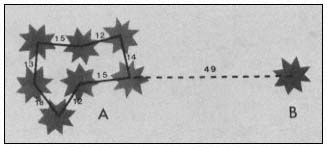
Figure 2.
A: A structural-group with plants of a given kind and size that
are all separated by distances that fall within the spatial-class.
B: A single-plant that is separated from other plants of the
same kind and size by a distance that exceeds the upper
limit of the spatial-class.

25-ft. The trees at the common margin can be less than 10 ft. from alder on one side and greater that 10 ft. from alder on the other side. In such cases, a rule must be used to assign plants of potential dual structural-group membership to one of the structural-groups. We assign such plants to the group with the narrowest spacing (see A, fig. 3).

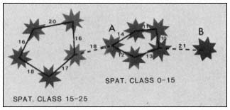
Figure 3.
A: A plant that could belong to more than one structural-group
because the distance between it and one or more other plants
of the same kind and size falls within one spatial-class while
the distance between it and one or more other plants falls
into another spatial-class. B: A plant that is recognized as a
single-plant because the distance between it and another
plant of its kind and size exceeds the upper limit of the
spatial-class for the structural-group to which the other
plant belongs even though the distance between the
plant and the other falls within the spatial-class used
in defining another kind of structural-group.

Structural-groups are assigned trinomial names consisting of a) the size-class; b) the species or growth-form of the compound plant-descriptive-class; followed by c) the spatial-class. In the description, species names are abbreviated by the first two letters of the genus and the species. The species growth-form is indicated by the combination of uppercase and lowercase letters. For tree species, uppercase is used for both the genus and species. For shrub and vine species, uppercase is used for the genus and lowercase for the species. For graminoid and forb species, lowercase is used for both the genus and the species. A structural-group consisting of 20- to 40-ft. tall cottonwood (Populusfremonti ) within 20 ft. of each other, for example, is referred to as: 20-40' POFR—0-20'.

In contrast to a structural-group, a single-plant is: a) a plant that is separated from any other plant in the same compound plant-descriptive-class, by a distance that exceeds the upper limit of the spatial-class that is used to define the structural-group with the widest spacing to which plants in that compound plant-descriptive-class are assigned (see B, fig. 2); or b) when more than one spatial-class is used with one compound plant-descriptive-class to define two or more kinds of structural-groups, it can also be a plant that is separated from any neighbor in the same compound plant-descriptive-class by a distance that exceeds the upper limit of the spatial-class of the structural-group to which its neighbor belongs (see B, fig. 3).

Single-plants are assigned a binomial name consisting of the compound plant-descriptive-class to which the plant belongs. For example, a single 20- to 40-ft. tall cottonwood plant that is more than 20 ft. from another is referred to as: 20-40'POFR.

Bounding Structural-Groups and Single-Plants

Structural-groups always have exterior boundaries, and they have interior boundaries as well when holes occur. These boundaries are based on crown projection boundaries of selected plants in the group. Since many projections are irregular because branches protrude at odd angles and differ in length, projections can be better bounded with polygons than with circles. To establish unequivocal boundaries for crown projections, we always use the smallest possible convex polygon^[6] that has vertices located at the tips of the longest branches (see A, fig. 4).

The first approximation of the exterior boundary of a structural-group is a convex polygon whose vertices are those of the crown projection boundaries which when connected form the smallest possible polygon that includes the crown projections of all plants in the group (see B, fig. 4). This approximation constitutes the structural-group boundary unless the distance between one or more pair of plants tangent to the first approximation boundary exceeds the upper limit of the spatial-class. Each new section of the boundary is formed by connecting vertices of crown projection boundaries to produce the

[6] A convex polygon is one in which all the interior angles are less than 180°.

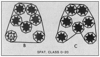
Figure 4.
A: The boundary of the crown projection of a plant.
B: A structural-group bounded by a convex polygon.

shortest boundary that includes the crown projections of all the plants in the group (see C, fig. 4). In the event that these criteria can be satisfied by connecting more than one set of crown projection boundary vertices for a section, the boundary for the section is established by connecting all the vertices that could be used to establish new boundaries for the section.

A structural-group has one or more interior boundaries when a hole(s) exists, giving the structural-group a doughnut shape or swiss-cheese appearance. A hole exists when the following two conditions are met: a) an area exists between plants that is large enough to accommodate a circle with a diameter greater than the upper limit of the spatial-class used in defining the structural-group; and b) the area is not completely covered by the crown projections of plants in the group (see C, fig. 4).

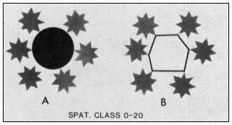
Figure 5.
A: A structural-group with a hole.
B: The boundary of a hole.

The boundary of a hole is a polygon which is formed by connecting vertices of crown projection boundaries of plants on the perimeter of the hole to produce the smallest possible polygon  (see B, fig. 5). The polygon can be either convex or concave.^[7]

Bounding Single-Plants

The boundary of a single-plant is simply its crown projection boundary (see A, fig. 4).

Spatial-Aggregations and Solitary-Plants

Structural-groups and single-plants overlap in such a wide variety of combinations in a vegetation that few locations can be expected to have the same combinations of structural-groups and single-plants. Consequently, if a general description of a vegetation were to be developed on the basis of these combinations, classes to which different combinations of structrual-groups and single-plants could be assigned would generally be so broad that the resolution obtained by recognizing structural-groups and single-plants would be lost and their recognition would have served no useful purpose.

Therefore, instead of assigning different combinations of structural-group and single-plants to classes, we assign only those structural-group(s) and/or single-plant(s) present at each location that include plants in the largest size-class to classes. Our rationale for giving priority to the largest plants at each location is that they are the dominant structural components in the vegetation, and in addition they occupy the largest part of the growing space and to a large extent control the environments of the plants growing beneath them.

All the structural-groups and single-plants, or portions thereof, that have the highest priority at any location are referred to as "spatial-aggregations" and "solitary-plants." Thus, a spatial-aggregation is a structural-group or portion thereof that is not overlapped by structural-groups or single-plants of higher priority; and a solitary-plant is a single-plant or portion thereof that is not overlapped by single-plants or structural-groups of higher priority.

Plants in the understory are not ignored in the description, however, when they are judged to be significant. Information about them can be collected in the inventory of spatial-aggregations and solitary-plants and included in the description as a descriptive variable after the spatial-class. Thereafter, the descriptive variable is used to further define the classes to which spatial-aggregations and solitary-plants are assigned.

To identify spatial-aggregations or solitary-plants, the overlap among structural-groups and single-plants must be allocated. This allocation is based on the priority assigned to

[7] A concave polygon has one or more interior angles that are greater than 180°.

these spatial units except when they have the same priority. Then the area of overlap is viewed as a mixture of spatial-aggregations and/or solitary-plants. The highest priority is assigned to structural-groups and single-plants that are defined, in part, by the largest size-class. Thereafter, successively lower priorities are assigned to structural-groups and single-plants that are defined, in part, by successively smaller size-classes.

These priorities are applied when allocating overlap as follows.

(a) The overlap among structural-groups of different priorities is allocated to the structural-group with the highest priority (see A, fig. 6).

(b) The overlap among single-plants of different priorities is allocated to the single-plant with the highest priority (see B, fig. 6).

(c) The overlap among structural-groups and single-plants of different priorities is allocated to whichever one has the higher priority (fig. 7).

(d) The overlap among structural-groups of the same priority is recognized as a mixture of spatial-aggregations (see A, fig. 8).

(e) The overlap among single-plants of the same priority is recognized as a mixture of solitary-plants (see B, fig. 8).

(f) The overlap among structural-groups and single-plants of the same priority is recognized as a mixture of spatial-aggregations and solitary-plants (see C, fig. 8).

The boundaries of spatial-aggregations, solitary-plants, or mixtures include boundaries of portions thereof of the spatial unit(s) from which they are derived. When the spatial-aggregation or solitary-plant is derived from a structural-group or single-plant that is not overlapped by one or more spatial units of higher priority, the boundary is that of the spatial unit from which the spatial-aggregation or solitary-plant is derived (fig. 6 and fig. 7). When the spatial-aggregation or solitary-plant is derived from a portion of a structural-group or single-plant, the boundary consists of a portion of the boundary of the spatial unit from which it is derived plus portions of boundaries of other structural-groups and/or single-plants (fig. 9). When a mixture is recognized, the boundary consists of the portions of the spatial unit boundaries that define the area of overlap (fig. 8).

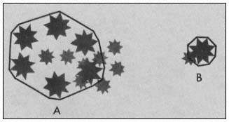
Figure 6.
A: A spatial-aggregation derived from the structural-
group with the higher priority. B: A solitary-plant
derived from the single-plant with the higher priority.

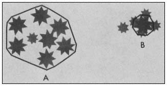
Figure 7.
A: A spatial-aggregation derived from a structural-group
that has higher priority than the single-plant it overlaps.
B: A solitary-plant derived from a single-plant that has
higher priority than the structural-group it overlaps.

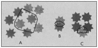
Figure 8.
A: A mixture of spatial-aggregations in the area of overlap
of two structural-groups with equal priority. B: A mixture
of solitary-plants in the area of overlap of two single-plants
with equal priority. C: A mixture of a spatial-aggregation
and a solitary-plant in the area of overlap of a structural-
group and a single-plant with equal priority.

Spatial-aggregations, solitary-plants, and mixtures are all named after the spatial units from which they were derived.

Description Method

As discussed, the description method is based on the recognition of vegetation units at two levels of resolution; and therefore, the description has two parts. The first provides a delineation of the different types of strata on an aerial photo or vegetation map along with a family of proportions that specifies the proportion of the area that is covered by strata of

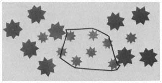
Figure 9.
The boundary of a spatial-aggregation that is derived from
only a portion of a structural-group. It consists of portions
of the boundary of the lower priority structural-group and
an portion of the boundary of each of the two higher
priority structural-groups.

each type. Unlike the description method presented by Bonnicksen and Stone (in press), however, the second part provides a family of proportions that specifies the proportion of the area covered by strata of each type that is covered by spatial-aggregations and solitary-plants of each type instead of visually determined aggregations.

Procedure

1. Obtain stereo pairs of aerial photos. Most often, a scale of 1:15,000 or larger is required if the proportion of different kinds of spatial-aggregation and solitary-plants recognized within strata of each type are to differ significantly.

2. On the photos, identify strata based on plant growth-form, species, growth-form-size, species-size, or some combination of these plant-descriptive-classes.

3. Determine the proportion of the area occupied by the vegetation that is covered by strata of each type using a planimeter or by sampling on the photo. As part of the description, organize these proportions as a family of proportions of stratum types. When desired, include the confidence interval for each proportion in the family of proportions if the proportions were estimated by sampling.

4. Decide which compound plant-descriptive-classes and spatial-classes will be used to define different types of structural-groups and single-plants.

5. Decide if any descriptive variables will be used to redefine the spatial-aggregation and solitary-plant types.

6. Design an appropriate sampling procedure for inventorying spatial-aggregations and solitary-plants within strata of each type. The sampling method that is most efficient in strata of a given kind depends on their size, the sizes of aggregations belonging to the most common aggregation type, and the ease with which one can move through the vegetation (Stromberg 1980).

7. Conduct field sampling at which time the spatial-aggregation, solitary-plant, or mixture at each sample point is identified as follows:

(a) Among the plants around or over the sample point, identify those that belong to the structural-group(s) and/or the single-plant(s) of highest priority that on first inspection appears to cover the sample point.

(b) Bound only enough of each structural-group or single-plant to determine whether or not it covers the sample point. If none does, identify structural-group(s) of successively lower priority until one or more is found that covers the sample point.

(c) Identify the spatial-aggregation(s) and/or solitary-plant(s) from among those structural-groups and/or single-plants that were found to cover the sample point by allocating any overlap or recognizing a mixture. If a descriptive variable is being used, collect the necessary information at each sample point.

8. Estimate the proportion of the area occupied by strata of each type that is covered by spatial-aggregations and solitary-plants of each type. As part of the description, organize these proportions as a family of proportions of spatial-aggregations and solitary-plant types. When desired, include the confidence interval for each proportion in the family of proportions.

Remarks

In a subsequent paper, L.P. Stromberg and E.F. Katibah will present an example of the use of spatial units with this method to describe a riparian vegetation.

Literature Cited

Bonnicksen, T.M., and E.C. Stone. In press. Reconstruction of a presettlement giant sequoia-mixed conifer forest community using the aggregation method. Ecology.

Fosberg, F.R. 1961. A classification of vegetation for general purposes. Trop. Ecol. 2:1–28.

Kershaw, K.A. 1964. Quantitative and dynamic ecology. 100 p. Edward Arnold Publishing Co. Ltd., London.

Stone, E.C. 1977. Timber management handbook. USDA Forest Service, Region 5, San Francisco, California, USA. Chapter 1. Stand management prescriptions. P. 1–40.

Stromberg, L.P. 1980. Relative cost-effectiveness of points, point clusters, and line transects in sampling vegetation for aggregation type proportions. Ph.D. Dissertation. 185 p. University of California, Berkeley.

An Application of the Spatial-Aggregation Method to the Description of Riparian Vegetation^[1]

Laurence P. Stromberg and Edwin F. Katibah^[2]

Abstract.—The spatial-aggregation method is used to resolve complex riparian vegetation into a mosaic. A vegetation survey produced a mosaic of 65 spatial-aggregation and solitary-plant types, eleven of them covering half the area surveyed. This paper outlines the survey methods used and hypothesizes some dynamic relationships between and within selected types.

Introduction

This paper demonstrates an application of the spatial-aggregation method developed and described by Stone etal . (1983). It describes the steps taken to estimate the proportional (relative) areas within a selected riparian study area occupied by each of several tree-and shrub-dominated spatial-aggregation and solitary-plant types. To illustrate the use of the method in characterizing overstory-understory relationships, understory tree and tree reproduction data were collected in each spatial-aggregation type represented in the study area.

Change in any vegetation, including riparian vegetation, is the cumulative expression of changes that result from local deaths of some plants, establishment and growth of others, and associated plant and group replacement processes. Due to differences in: 1) the kinds, intensities, areal extent, and timing of disturbances; 2) the sources, amounts, and distribution of seed; 3) the successful establishment and subsequent growth of constituent species; and 4) other variables affecting vegetational development, a variety of overstory-understory relationships and species combinations normally exist in any riparian zone. Riparian vegetation is typically both compositionally and structurally heterogeneous. Therefore the change that takes place over the whole during a given time interval is likely to be a composite product of local changes proceeding at different rates and in different directions.

When data are combined, averaged, or otherwise synthesized across a vegetation which has in the past, or is in the future, likely to change along multiple successional (and other) pathways, two undesirable outcomes can result. First, the data summary or description may not portray the conditions that underlie the range and variety of types of changes possible. It may represent the full range of variation, a desirable feature, but it may not indicate that the heterogeneous whole is locally homogeneous, an undesirable feature if such homogeneity exists. Second, the data summary may obscure important differences in those overstory-understory and horizontal-spatial relationships between plants which partly drive and explain the multiple change potentials.

Under these conditions, the vegetational description has a low level of resolution, making it less useful than it could be as an analytical or management tool. Vegetational resources and processes are understood not on the basis of their actual character, but on the basis of information about that character gained from collecting data and generating descriptions. If the resource is very complex, patchy, or can be readily recognized as a mosaic, and if it changes in a non-uniform manner over space and time, data should be collected and organized to portray the mosaic and the associated various changes possible. Ecologically significant or substantial differences should be represented in the description—data should not be amalgamated across them.

The spatial-aggregation method allows users to arbitrarily but meaningfully and quantitatively treat vegetation as a mosaic, when that approach is warranted, and to describe the smaller, more homogeneous groups of plants which create the heterogeneous whole. The user incor- porates the desired degree of resolution into data collection and description. This resolution is normally higher than that characteristic of most largearea vegetation surveys. By virtue of the focus on smaller homogeneous units, observations are

[1] Paper presented at the California Riparian Systems Conference. [University of California, Davis, September 17–19, 1981].

[2] Laurence P. Stromberg is Associate Project Manager with Larry Seeman Associates, Inc., Berkeley, Calif. Edwin F. Katibah is Associate Specialist, Department of Forestry and Resource Management, University of California, Berkeley.

directed into areas in which environmental variation and the plant responses to that variation are relatively narrow. This focus simplifies both analysis of the vegetation and the prediction of change.

Study Area

The Las Trampas Creek study area is approximately 11.3 km. (7 mi.) east of Berkeley, Alameda County, and 3.2 km. (2 mi.) south of Lafayette, Contra Costa County. The area surrounding the riparian zone was at one time farmed, grazed, and planted in pear, plum, and walnut orchards. Today the area is suburban—much of the agricultural land has been converted to residential development. At Las Trampas Creek, residential development has occurred right into the riparian zone, causing the partial elimination and local destruction of the natural vegetation that once lined the watercourse.

Las Trampas Creek is incised into alluvial material mapped by the USDA Soil Conservation Service (SCS) (1977) as Clear Lake clay. Currently, the channel bottom is 7.5-12 m. (25-40 ft.) below the level of the upper terrace. Locally, one or two minor intermediate terraces are also present. These are distinguishable from benches produced by slumping and oversteepening of terrace banks.

The vegetation along Las Trampas Creek has retained much of its natural character, but, at the same time, the impacts of suburbanization and associated disruptions were evident. Fremont cottonwood (Populusfremontii ), white alder (Alnusrhombifolia ), and two willows (Salixlaevigata and S . lasiandra ), all common tree species in the central coast riparian forest according to Roberts etal . (1977), were present in the overstory of the study area. Bigleaf maple (Acermacrophyllum ) and black walnut (Juglanshindsii ), both less common tree species, were also present. The walnut had, however, probably grown from seed produced in abandoned walnut orchards adjacent to the creek. At one time in the Walnut Creek-Lafayette area, English walnut (J . regia ) was grafted onto black walnut rootstock to improve the quality of the walnut crop. When the walnut industry declined, the orchards were left untended and the tree tops died or were overtaken by sprouts from below. Subsequent seed produced was from the black walnut rootstock—this was the likely source of the walnut in the study area. Other tree species present included California bay (Umbellularia californica ), coast live oak (Quercusagrifolia ), valley oak (Q . lobata ), California buckeye (Aesculuscalifornica ), and box elder (Acernegundo ).

Among the more abundant shrub species in the study area were wild blackberries (Rubusursinus and R . vitifolius ), elderberries (Sambucus spp.), wild rose (Rosacalifornica ), gooseberries (Ribes menziesii and R . divaricatum ), and river snowberry (Symphoricarposrivularis ). Several willows not identifiable to species at the time of the field survey were also present in the study area. Common vines included Dutchman's pipe vine (Aristolochiacalifornica ), clematis (Clematisligusticifolia ), poison oak (Rhusdiversiloba ), and the introduced and escaped English ivy (Hederahelix ).

Methods

The essential steps in designing the field survey were: a) choosing what kinds of structural groups would be recognized; and b) selecting the types of sampling units to be used in estimating spatial-aggregation type proportions and collecting understory tree and tree reproduction data.

Structural Group Selection

Structural groups are basic building blocks from which a mosaic of spatial-aggregations is conceptually organized. In this study, they are defined and recognized on the basis of species or life form, plant height, and plant spacing.

Plant descriptive classes and spatial-classes can be defined a several ways. Whenever ecological information is available it can be used; whenever objectives are clearly stated they should be used as well. Growth data and estimates of the greatest attainable height for each species given the site conditions within the study area can be used to define height-classes. These classes can be the same or different for each species. Pattern studies or previous investigations into the effects of density on height or diameter growth can be used to set spatial-class limits. In the absence of such information, qualitative, semi-quantitative, or fully quantitative methods can provide the means for setting limits on spatial-classes.

An investigator can rely on past experience to set the limits for height- and spatial-classes and make no measurements at all. Such an approach would be acceptable if the product of the investigation met the needs of the user. Qualitative and quantitative methods of any kind can be used. One possible quantitative method uses a distance measure such as the wandering quarter method (Catana 1963) to obtain a sample of nearest-neighbor distances for plants belonging to the same compound plant descriptive class. Height-classes could be established prior to or during the distance sampling.

In this study, we relied upon the visual discontinuities in the vegetation, that is, its visible patchiness, as the basis for establishing the structural groups we would recognize. During two trips through the length of the study area, tree heights and spacings in a large number of visually recognizable plant groups were measured. We chose to measure height rather than diameter

to facilitate a simpler portrayal of overstory-understory relationships. We used distance between stems rather than between crowns (an acceptable alternative, particularly in shrubdominated vegetation types) because stem spacing is a visible and more easily measured variable.

We established at least two types of structural groups for each plant descriptive class and then conducted a trial run to determine how satisfactorily the structural groups we recognized resembled their "visual" counterparts in terms of plant membership. As expected, the match was imperfect, and a few minor adjustments in the height- and spatial-classes were made to improve the "fit". Partial coincidence between certain abrupt visual discontinuities and structural group and spatial-aggregation boundaries is normal, particularly when the visual mosaic is used to set height- and spatial-class limits, but some differences will persist. Plants that appear to warrant inclusion in a structural group because of their taxonomic identity are sometimes excluded because they are too tall, too short, or too far away from their nearest like neighbor to be included.

Imperfect registration or coincidence between visible patches in the vegetation and spatial-aggregations is unavoidable if the strict rules for deciding upon structural group membership and boundary location are followed. The user must accept the associated discomfort with the understanding that the consequences are repeatable sampling results and essentially identical boundary allocations, even by field survey teams working independently—the discrepancies should amount to no more than crown projection and measurement errors.

Table 1 contains the height- and spatial-classes used in recognizing structural groups and some examples of structural group trinomial names. By convention, plants whose heights placed them at height-class boundary limits were considered members of the "taller" of the two adjacent height-classes. In other words, the classes were handled in the field and in subsequent analyses to be 0.0–0.29, 0.3–0.89, 0.9–1.79, etc. The same convention was applied to plant spacing.

Non-overlapping, mutually exclusive height-classes were used to facilitate representation of overstory-understory relationships. The same height-classes apply to all species. Several of the species occurring in the study area, including cottonwood, the several willows, alder, and others, sprout; consequently some means had to be established to provide for unambiguous measurement of distances between multi-stemmed plants. By convention, distance was measured from the geometric center of the stem cluster. When required, a hole was dug to permit measurement.

Species were used to recognize all tree, shrub, and vine structural groups. However, forbs were not identified to species and forb structural groups were recognized on the basis of life form.

Sample Survey Design

Approximate limits to the study area were set using color aerial photographs flown at a scale of 1:3,000. Three adjacent photographs from a single flight line provided complete coverage. Although we could have stratified the vegetation prior to sampling by coupling a minimal amount of photo-interpretation with ground verification, we chose not to because the study area is small and we did not intend to map the vegetation. For sampling purposes, we set the actual limits of the study area at 15.2 m. (50 ft.) from the edge of the upper terraces. The setback was used to include trees rooted above the terrace but belonging to spatial-aggregations containing trees rooted between the terraces.

Single points were used as the sampling units. They were randomly located to yield the largest possible sample size. By grouping points into clusters, total sampling time could be reduced. However, this would significantly

decrease the precision possible in the estimated type proportions. Computer-generated random points were plotted onto mylar sheets. These sheets were placed over the three aerial photographs and points were transferred by pin from the mylar to the photographs. The point number, plotted beside the point on the mylar sheet, was marked on the back of the photograph to identify the point and insure that subsequent associations of field data with sampling locations would be correct.

During the field survey, points were thrown out of the sample whenever they fell in vegetation heavily modified by residential landscaping or local trash disposal. These points were replaced by others located elsewhere in the study area. The results are thus biased—dumpsite and unnatural vegetation are underrepresented in the sample. However, the number of points relocated was minor compared to the total sample size and the bias was therefore neglected.

Data on understory trees and tree reproduction were collected in square quadrats. Three-meter-square quadrats were used in tree-dominated aggregations, two-meter-square quadrats were used in shrub- and vine-dominated aggregations, and one-meter-square quadrats were used in forb-dominated aggregations. Quadrat size was reduced to insure that the quadrat could fit entirely within the limits of the spatial-aggregation recognized; smaller quadrats are necessary as the size of the dominants and the area of the associated spatial-aggregation decreased. In most instances, the quadrat was placed at the sample point location. Occasionally, however, when the point was near the boundary of the spatial-aggregation, it was relocated toward the center of the spatial-aggregation to avoid quadrat overlap. Whenever the spatial-aggregation was too small to contain the quadrat, the area of the spatial-aggregation was measured, and this was used in lieu of a quadrat—all trees and tree reproduction were counted within the spatial-aggregation boundary. Understory tree and tree reproduction data were collected using the same height-classes as for the structural groups.

Each quadrat was identified as to site and described by location (upper terrace, intermediate terrace, lower terrace, inter-terrace slope, slump, channel bottom, etc.). In addition, occular estimates of the total groundcover present in each quadrat were made using Daubenmire's (1968) cover classes, and the most abundant ground layer species were identified.

Sample Statistics

When sampling with randomly located points, the estimator for the proportion, P_i ., of the "ith" spatial-aggregation or solitary-plant type is:

An unbiased estimator of the variance of P_i obtained from the sample is:

Confidence Limits

Placement of a confidence interval around a proportion with a stated alpha level, 0.05 for example, assumes reliance upon the normal approximation in the 95% confidence statement that the interval contains the true proportion. With an alpha level of 0.05 we accept that five out of 100 confidence intervals will not contain the true proportion and that we will have erred in those cases. As the number of estimates for which we produce confidence intervals increases, the overall error rate increases. With an alpha level of 0.05 for each of 10 intervals, the overall error will be somewhere between 0.05 and 0.50 but will be undefined. We can preserve an error rate with a definable upper limit of 0.05 by using simultaneous multinomial confidence intervals, each with an alpha level of 0.005. The result is wider confidence intervals.

Multinomial confidence limits to the intervals about estimates obtained for spatial-aggregation and solitary-plant proportions p_i ., i = 1,2,3 . . . c, using a sample of randomly located points are:

where   = chi square with one degree of freedom and a significance level of ,     = the overall acceptable error rate, and c = the number of types over which the overall acceptable error rate is to be preserved.

Results and Discussion

Table 2 shows the estimated spatial-aggregation and solitary-plant type proportions.

These proportions and the confidence intervals about the largest individual and combined type proportions shown in table 3 are based on a sample of 192 randomly located points. Together, the tables show the predominance of willow spatial-aggregation types; the three most abundant types contained either Salixlasiandra or S . laevigata , and had a combined proportion of .182, indicating that these spatial-aggregation types occupied just over 18% of the study area. Figure 1 (left) shows a willow spatial-aggregation with 12.2- to 20.9-m. tall trees with nearest neighbor distances less than 2.5 m. Such spatial-aggregations were found on lower terraces and the thick sediment layers deposited during past floods.

The next two most abundant spatial-aggregation types were 1.8–3.7 BApi 0.0–2.0 and 3.7–6.1 SALA 0.0–2.5, with proportions of .052 and .037, respectively. The latter type is shown in figure 1 (right). These spatial-aggregation types occurred in quite different environments, the coyote brush primarily at the edge of the upper terrace and on slumps and in their scarps; the willow primarily along the stream channel and less than 1.5 m. (5 ft.) above it.

Alder, buckeye, black walnut, and willow spatial-aggregation and solitary-plant types were next in order of abundance and area covered. Each type accounted for slightly over 3% of the study area. Figure 2 shows a 12.2- to 20.9-m. tall solitary alder in the left foreground and two alder spatial-aggregations, 6.1–12.2 ALRH 0.0–3.0 in the left-center middleground and 12.2–20.9 ALRH 3.0–8.7 in the right middleground.

As table 3 shows, mature solitary alder, willow, and black walnut were common—in most cases the willow and alder standing alone because their neighbors had died or suffered crown damage

which placed them in a shorter height-class. Black walnut, on the other hand, occured primarily as solitary, pre-mature individuals. In fact, three-quarters of the walnut trees represented in the sample occurred solitarily, even in the shorter height-classes.

Figure 1.
Willow spatial-aggregations abundant in the Las Trampas Creek riparian woodland. Left—12.2–20.9 SALA 0.0–2.5,
a dense aggregation of mature trees. Right—3.7–6.1 SALA 0.0–2.5, a dense aggregation of immature trees.

Figure 2.
A combination of a solitary alder 12.2–20.9-m. tall (left
foreground) and alder spatial-aggregations, 6.1–12.2
ALRH 0.0–3.0 (left-center middleground) and
12.2–20.9 ALRH 3.0–8.7 (right middleground).

Eleven of the 65 spatial-aggregation and solitary-plant types encountered in the survey have a combined proportion of .458 and cover just under one-half of the study area. Among the remaining types, willow tree and shrub types are most abundantly represented.

A mosaic of spatial-aggregations is formed when structural groups overlap one another. This is particularly true in multi-layered vegetation such as is commonly found in riparian zones. In the study area, this overlap is the rule. Most structural groups straddle spatial-aggregation boundaries and few spatial-aggregations do not contain parts of several shorter structural groups. The survey results nevertheless indicate that despite the overwhelming amount of structur-

al group overlap, over 97% of the study area consists of pure, single-species spatial-aggregations. This suggests that most of the overlap occurs between structural groups with different height-classes.

The relatively small proportion of the study area in mixed spatial-aggregations suggests that it is possible to recognize visually homogeneous patches and to use them as a basis for quantitatively organizing vegetation into a mosaic of distinguishable units. Of course a mosaic of spatial-aggregations is an artifact of height and spatial-classes combined with species to define structural groups. Each particular combination will yield a unique mosaic. Nevertheless, the results indicate that the spatial-aggregation method can be used to partition even complex, heterogeneous riparian vegetation into definite, locally overstory-homogeneous units in a very simple manner. These units or spatial-aggregations then become the focal points of resource analysis and evaluation of past and potential future change.

Figure 3 diagrams some hypothetical dynamic relationships between several willow spatial-aggregation and solitary-plant types. The assumption of a relationship constitutes substitution of space for time. The arrows indicate possible trends from shorter, denser spatial-aggregations to taller, less dense spatial-aggregations. The structural transitions ultimately would terminate with solitary-plants. These developmental pathways are considered here without regard for past or future successional (compositional) changes which may be foreshadowed by understory trees and tree reproduction of other species.

Figure 3.
Hypothetical relationships between willow spatial-aggregations
and solitary-plants in a natural thinning process.

The several pathways suggest the kinds of essentially structural change in spatial-aggregations which could follow flooding—the abrasion, destruction, and/or removal of the previous cover, the deposition of a new unoccupied substrate, and the subsequent establishment and growth of willow from seed. Over time, the initially dense spatial-aggregations of shorter willow would undergo natural thinning. Some trees would die; growth would be transferred to the survivors which would eventually form taller, less dense spatial-aggregations. A decrease in the number of stems in each spatial-aggregation would accompany the losses through mortality. In the absence of disturbances severe enough to initiate this same developmental sequence elsewhere in the mosaic, a shift would occur in the areas occupied by spatial-aggregations representing early and later developmental stages. The taller, open spatial-aggregations would eventually occupy a greater proportion of the mosaic.

The ultimate transition to solitary trees could result from the death of some of the older willow in the mature spatial-aggregations. Since mortality would thin spatial-aggregations that already contained a reduced number of trees, the outcome could be a residual of several old, solitary individuals that together formed part of the same shorter spatial-aggregation several decades earlier, standing apart from each other.

These changes can be described a number of ways. Using the spatial-aggregation method, they are captured as the movements of groups of plants from one spatial-aggregation type to another. This suggests that structural group and spatial-aggregation membership and boundaries are transitory mosaic characteristics that change over time as plants grow in response to the environments they encounter. Groups form, spatial-aggregations coalesce and split apart, and type proportions increase and decrease, some to zero as types temporarily or permanently drop out of the mosaic.

In figure 3, the parentheses below each type contain the number of sample points that occurred in each type of spatial-aggregation, giving a relative indication of how much area is occupied by each representative of these hypothetically related developmental stages. If this scenario can be considered a realistic possibility for the study area, the data from the survey indicate that the relatively early stages are heavily represented and that very dense, mature willow spatial-aggregations are not very common.

The thinning processes hypothesized above are now evident in the study area. Several neighboring spatial-aggregations of the same type appear to have once formed a single larger predecessor. Dead and unhealthy trees slightly shorter than their live neighbors now separate these neighboring spatial-aggregations. This splitting has apparently accompanied the death or decline of the slowest-growing individuals in what were initially very dense spatial-aggregations.

During the field survey we recorded the number of trees in each spatial-aggregation sampled. Using the number of trees in a spatial-aggregation as a measure of its size, we found that although the sample of quadrats is too small

to permit a meaningful test of the statistical significance of the differences, trends in spatial-aggregation size tentatively support the above hypothesis. As the height-class increases, the average number of trees in willow spatial-aggregations decreases. For types with a spatial-class of 0.0–2.5 m., the decrease is from 12.3 to 8.2 to 6.1 trees per spatial-aggregation. Similarly, a decrease from 5.1 to 3.0 stems per spatial-aggregation was found between 6.1–12.2 SALA 2.5–6.7 and 12.2–20.9 SALA 2.5–6.7.

The trend in reduction in tree numbers is more evident between types that vary in spatial-classes. For 6.1- to 12.2-m. tall spatial-aggregations, those with 0.0- to 2.5-m. stem spacing average 12.3 trees, those with 2.5- to 6.7-m. stem spacing average 5.1 trees. In 12.2- to 20.9-m. tall spatial-aggregations, the average decreases from 8.2 to 3.0 trees as the spacing increases. This pair of trends better captures the thinning possible.

Although our data will be used to set several hypotheses for future work, the purpose here is not to test hypotheses about the above structural dynamics. Relationships are discussed here solely to indicate the ways in which vegetation dynamics can be tracked using the spatial-aggregation method.

Replacement processes whereby groups of plants belonging to one species replace those of another, either by mortality of the original species, or as the replacement species grows through them and assumes vertical dominance, can also be portrayed at a high level of resolution. The understory tree and tree reproduction data collected in each spatial-aggregation type suggest species replacement processes, including successional change. To illustrate the possibilities in mature alder spatial-aggregations we have combined data from the plots in 12.2–20.9 ALRH 0.0–3.0 and 12.2–20.9 ALRH 3.0–8.7 types (fig. 4). Black walnut, California bay, buckeye, alder, and willow are present in the understories of these types of spatial-aggregations. In some cases, we suspect that the alder became established later and grew through the trees now in the understory, in others that the understory trees became established after the alder. We would need to core both overstory and understory trees to confirm our opinions. Some of the understory trees such as box elder and buckeye normally attain a height of only 10 m. and would form an overstory only in the event that the taller trees die or are removed in some way. Bay, black walnut, and willow, however, can replace alder without reducing the height of the overstory canopy.

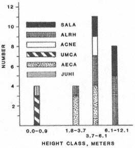
Figure 4.
Understory trees and tree reproduction in
12 3-m. × 3-m. quadrats in mature 12.2-
to 20.9-m. tall alder spatial-aggregations.

In some of the alder spatial-aggregations, shorter, younger alder is present in the understory, insuring that mature alder spatial-aggregations will remain in the mosaic in spite of future mortality. Of course, alder is also present under willow, cottonwood, and walnut spatial-aggregations and can replace the overstory trees in these too.

Figure 5 illustrates tree reproduction in 6.1- to 12.2-m. tall buckeye spatial-aggregations. These buckeye spatial-aggregations generally occur above 1.5 m. (5 ft.) above the stream channel and are common on the minor intermediate terraces. Contrary to the situation in the alder spatial-aggregations, no alder or willow reproduction is present. Valley oak, walnut, bay, and buckeye are present—the last are by far the most abundant. Buckeye seedlings (0.0–0.9 m.) and saplings (0.9–1.8 m. and 1.8–3.7 m.) appear to have grown from seed produced by the trees in the overstory. The other species have, of course, become established from seed produced by trees in neighboring spatial-aggregations. In one case, a buckeye spatial-aggregation surrounds a solitary bay 12.2–20.9 m. tall; the four bay seedlings and saplings represented in figure 5 all occur just beyond the

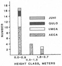
Figure 5.
Understory tree and tree reproduction
in five 3-m. × 3-m. quadrats in 6.1- to
12.2-m. tall buckeye spatial-aggregations.

crown of the solitary bay and beneath the buckeye. Whether or not the buckeye seedlings will survive to replace the overstory buckeye is uncertain. No seedling survival information is available.

Ideally, projection of change in and maintenance of buckeye spatial-aggregations requires data on seedling survival and seedling and sapling growth in buckeye spatial-aggregations. Seedling survival and growth both vary with differences in light reduction and water consumption by trees in the overstory. These, in turn, vary with the height of trees, their density, and crown closure. Success of reproduction no doubt varies across spatial-aggregation types.

Reproduction alone may not be sufficient to maintain the existing buckeye spatial-aggregations, even when reproduction is adequate and both seedlings and saplings are present in large numbers in the understories. Buckeyes are quite short; often buckeye spatial-aggregations are surrounded by taller trees. Upon full height growth these surrounding trees may overtop the buckeye from the side. Buckeye may continue to survive in understory structural groups, as it appears capable of doing in the study area. But once a buckeye spatial-aggregation is overtopped, either from the side or by trees growing through it, it may no longer retain its status as a spatial-aggregation. Using this method, only overstory mosaics are characterized.

Conclusion

By keeping track of overstory-understory relationships and insuring that data on the understory are collected in plots entirely within the boundaries of particular spatial-aggregation types, the investigator is able to predict local successional and other replacement processes not possible when data are merged across several types of spatial-aggregations. Many more kinds of change are identifiable. As a result, exceptions to commonly accepted successional scenarios can be recognized. The exceptions are, however, a matter of resolution. Higher levels of resolution and recognition of departures from standard beliefs are valuable steps in the direction of improving our grasp of the mechanics of vegetation change.

Although the potential user may consider this approach to involve too high a level of resolution for a large area survey, the level of resolution can be flexibly set by the user. As with traditional data collection and descriptive methods, data are collected over the entire target vegetation or survey area using this method. However, with the spatial-aggregation method the user can accomodate the visible heterogeneity and structural variation in a way that more satisfactorily accounts for their influence on vegetation dynamics. Still, no more time need be spent collecting data than would be required with traditionally accepted methods. Therein lie the potential advantages of using the spatial-aggregation method.

Literature Cited

Catana, A. J., Jr. 1963. The wandering quarter method of estimating population density. Ecol. 44(2):350–360.

Daubenmire, R. 1968. Plant communities, a textbook of plant synecology. 300 p. Harper & Row, New York, N.Y.

Roberts, W.G., J. G. Howe, and J. Major. 1977. A survey of riparian forest flora and fauna in California. p. 3–19. In : A. Sands (ed.). Riparian forests in California: their ecology and conservation. Institute of Ecology Pub. No. 15, University of California, Davis. 122 p.

Stone, E.C., J.I. Cavallaro, and L.P. Stromberg. 1983. In : R.E. Warner and K.M. Hendrix (ed.). California Riparian Systems. [University of California, Davis, September 17–19, 1981.] University of California Press, Berkeley.

USDA Soil Conservation Service. 1977. Soil survey of Contra Costa County, California. 122 p. plus maps. USDA Soil Conservation Service, Washington, D.C.

Structural, Floristic, and Condition Inventory of Central Valley Riparian Systems^[1]

Richard E. Warner^[2]

Abstract.—At the time of European settlement of the Central Valley in the mid-1800s, between two and three million acres of seasonally inundated floodplain supported vast areas of both aquatic and riparian wetlands. Over 90% of the valley's riparian systems are now gone. This paper reports a ground-based inventory of 51 riparian sites, some randomly selected, others chosen for their special structural or ecological values. Morphological structure, floristics, plant diversity, and site condition were quantified using an inventory methodology designed for that purpose. Stem diameter size-frequency curves for major canopy species indicate major reproductive problems in several species. Condition trends are assessed, and human-use impacts are discussed.

Introduction

History of the Problem

Since the first establishment of Spanish land grants in the early 1800s, the riparian systems of California's Central Valley have experienced an unremitting assault from cultivated agriculture, pasture and open-range grazing, dams and water diversions, groundwater pumping, flood control engineering, fuel wood cutting, and other consumptive uses and development activities.

Little note was taken of the cumulative impacts of these activities until the mid-1970s, when conservationists belatedly realized: a) the immense ecological importance of riparian systems; and b) the magnitude of their loss. In California, field studies of human-use impacts (e.g., McGill 1975, 1979) and riparian conferences in 1976 and 1977 (Sands 1977) brought these values and the extent of the loss into some perspective. During the same period, authoritative reports and the proceedings of important riparian conferences were emerging across the land, documenting the unusual importance of riparian systems as wildlife habitats, as protectors of the hydrologic and ecologic integrity of streams, as major recreation sites, and potentially as major forest product resources (e.g., Anderson and Ohmart 1977; Carothers et al . 1974; Gaines 1977; Hubbard 1977; Jain 1976; Johnson etal . 1977; Johnson and Jones 1977; Korte and Frederickson 1977).

California Riparian Study Program

In 1978, goaded by now-alarmed conservationists, the California Legislature enacted legislation (AB 3147, Fazio) mandating and funding a study of Central Valley and California Desert riparian resources by the California Department of Fish and Game (DFG). The stated goal of DFG in mounting its California Riparian Study Program (CRSP) was: "to protect, improve, and restore the riparian resources of the state." Specific objectives were:

1. To determine the historical extent of the riparian resource in the Central Valley and California Desert and the causes of its destruction;

2. To determine the present status of the riparian resource;

3. To identify problems and threats to resource maintenance;

4. To recommend measures for riparian resource protection, improvement, and restoration."

The above goal and objectives were essentially the same as those which guided the Department's successful coastal wetland program. (Warner 1979)

[1] Paper presented at the California Riparian Systems Conference. [University of California, Davis, September 17–19, 1981.]

[2] Richard E. Warner is Director, Field Studies Center, Davis, Calif.

The CRSP studies began in 1979. The first, a riparian vegetation mapping project of Central Valley depositional bottomland, using California Department of Water Resources (DWR) 35mm. aerial photographs, was undertaken jointly by the Departments of Geography at California State University, Chico, and California State University, Fresno (Central Valley Riparian Mapping Project 1979). The second project was a problem analysis and research planning effort undertaken by the Field Studies Center, Davis (Warner 1979). The third project, a riparian mapping and inventory design study, was undertaken by the Remote Sensing Research Program, Department of Forestry and Resource Management, University of California, Berkeley (Bonner etal . 1979). These were followed in 1980 by a two-part, collaborative field inventory and condition assessment. Two research teams—Remote Sensing Research Program, University of California, Berkeley, and Field Studies Center, Davis—undertook, respectively, remote-sensing and ground-based inventories of selected Central Valley riparian systems. This paper reports some of the findings of the ground-based inventory component of the CRSP.

Objectives and Constraints

It was recognized at the outset that a definitive ground-based study was not possible, owing to: a) the vast size of the study area (8.3 million hectares); b) limited resources ($20,000, of which $15,000 was provided by the Denver Wildlife Research Center, USDI Fish and Wildlife Service [FWS]); c) limited time (four months field time for ground-based studies); and perhaps most important, d) lack of prior studies of Central Valley riparian systems. With the exception of Conard etal . (1977) and Roberts etal . (1977), virtually no quantitative studies of the morphological structure of riparian vegetation and its floristics had yet been undertaken. No quantitative information on regional differences had been developed. California riparian plant associations and communities were only partly defined. No riparian classification system had been developed. And no standardized field procedures specific to riparian systems had yet been developed.

Limited time and the need to develop and test quantitative procedures precluded extensive preliminary sampling to determine study site stratification possibilities. Thus, the CRSP ground-based study of the Central Valley was designed as a first, broad-brush effort, where the objectives were to:

1) develop, test, and deploy a quantitative riparian inventory methodology;

2) describe and quantify the diversity of riparian system morphological structure, floristics, and condition; and

3) determine the major causes of condition decline and recent overt loss of riparian systems throughout the study area.

Structural, floristic, and other riparian system variables were selected based on what appeared to be real intra-system relationships and which were at the same time universal; that is, they were common to many kinds of riparian systems in many places. Randomized sampling procedures, other than site selection, were not attempted owing to the complete absence of quantitative information on intra-site and inter-site variance. It seemed more naive to make the pretense of known normal distributions and variances of as yet undefined plant association types, than to admit our ignorance and start at "square one" with the most rudimentary quantitations. The present study thus lays the groundwork for later stratification and randomization in sampling procedures.

The Study Area

Physiography

The Central Valley of California is an immense, flat-bottomed trough averaging 160 km. wide and comprised of two principal subunits, the San Joaquin Valley south of, and the Sacramento Valley north of the Delta. It extends in a northwesterly direction from its southern end near Bakersfield, Kern County, for some 830 km. It is bounded by four landform provinces: on the east by the Sierra Nevada; the south and west by the Coast Ranges; and on the north and northeast by the Klamath Mountains and Cascade Range (Durrenburger and Johnson 1976).

The Fazio legislation prescribed that the boundary of the Central Valley study area be at the upper edge of the blue oak/digger pine zone of Küchler (1977). This vegetation boundary lies at about 1,060 m. elevation in the south, gradually lowering to about 760 m. elevation in the north. It encompasses an area averaging 110 km. E–W and 750 km. N–S, or a total land area of approximately 82,500 sq. km. (8.25 million hectares or 20.3 million acres). The bottom of the trough, i.e., the valley floor, is comprised largely of unconsolidated sediments, ranging from about 1,000 m. of depth in the north to as much as 17,000 m. of depth in the lower San Joaquin Valley. These sediments provide a permeable matrix for an aquifer or groundwater storage basin which is by far the largest in the state.

Climate

Climate ranges from desert in the south and south-central portion, through steppe in the center, to warm summer Mediterranean in the north. Precipitation on the valley floor is as low as 127 mm. per year in the south, increasing to 760 mm. per year in the north. Precipitation in the surrounding hills and mountains is significantly higher, up to 2,000 mm. per year in certain northerly Sierra and Cascade parts of the watershed (Durrenberger and Johnson 1976).

Temperature patterns are somewhat unusual, in that both the far northern and far southern ends experience 90–120 days per year above 32°C (90°F), while the central portion receives but 60–90 days per year in that temperature range. In contrast, the surrounding foothills have on average but 30–60 days per year above 32°C. Winters tend to be mild throughout the Central Valley, with low clouds and fog ameliorating winter cold. Freezing temperatures occur principally from the influx of cold air from Canada in January and February (ibid .).

Fluvial Systems and Surface Hydrology

The watersheds and their draining streams and rivers on both sides of the Central Valley have common patterns of sediment transport, although those of the east side (the west slope of the Sierra) carry much more water. Eroded materials are transported down in steeply sloped, incised channels from the higher mountains, ultimately to be deposited on the broad, gently sloping alluvial fans comprising the lower termini of the watersheds. These alluvial floodplains, found along both sides of the valley floor at the bases of the mountains, tend to coalesce at their lateral margins with adjacent fans. The valley floor is thus a centrally depressed surface, the center of which is a sink with permanent wetlands, whose topography is in a slow but constant process of change from sequential alluvial depositions and the continued slow subsidence of the valley floor itself. Many Central Valley towns and cities (e.g., Sacramento, Fresno, Marysville, Yuba City, Bakersfield) are built on these alluvial floodplains and have experienced chronic flooding problems as a result. A more thorough treatment of Central Valley hydrology can be found in Katibah (1983) and Warner and Hendrix (in press).

It is difficult to generalize about Central Valley fluvial systems. They vary from small, first-order ephemeral streams to large, mainstem bottomland rivers. Prior to extensive water development, between 0.8 to 1.2 million hectares (2 to 3 million acres) of the valley floor were seasonally flooded, creating vast areas of floodplain riparian forest, woodland, savannah, and meadow. Duration of seasonal flooding varied from a few days to several months, depending on topography and on the timing and magnitude of storms and snowpack (Zeiner unpublished; California Department of Public Works 1931a,b).

In 1850 the U.S. Congress passed the Arkansas Swamp Act, permitting these "swamp and overflow lands" to be turned over to the states. In 1871, after much quarreling over where boundaries should be, the U.S. Secretary of the Interior accepted the State's determination of 887,654 ha. (2,192,500 ac.) of "swamp and overflow lands" (Thompson 1957; Zeiner unpublished). Somewhat later, the then-California Division of Water Resources, in Bulletins 26 and 29 (California Department of Public Works 1931a,b) concluded that in the Central Valley there were some 1,262,753 ha. (3,119,000 ac.) of floodplain bottomland subject to "seasonal or permanent flooding." This figure did not include the extensive riparian zones along tributary streams and rivers, which if included would raise the figure by at least another 300,000 ha. (740,000 ac.).

The significance of this is apparent. First, virtually all these seasonally inundated floodplain bottomlands were riparian wetlands. Second, based on both federal and state determinations, the historical extent of Central Valley riparian wetlands (as of 1871) was far greater than recent estimates based on reviews of early vegetation maps and present vegetation patterns (Roberts etal . 1977; Smith 1977; Katibah, Nedeff, and Dummer 1983; Küchler 1977). The influence of this vast complex of riparian wetlands upon Central Valley ecology was profound.

Surface hydrology and native vegetation patterns of the Central Valley have been greatly and perhaps permanently altered by human activities. Dams now block the flows of most of the larger streams and rivers, and, in so doing have massively altered the hydrologic regimes of the watercourses and associated groundwater basins. In some cases, the water so dammed is diverted out of the watershed altogether. Overbank flooding, siltation, and natural revegetation of the riparian zone have been greatly reduced. Thousands of kilometers of diversion ditches and canals now remove water from the streams, transporting it elsewhere for agricultural and other purposes, reducing groundwater recharge rates in the floodplains. In some areas, especially in the San Joaquin Valley, groundwater pumping from wells has lowered the water table to below root zones, rendering large areas uninhabitable to native trees and shrubs. The construction of thousands of kilometers of levees for flood control purposes has isolated hundreds of thousands of hectares of riverine floodplain from the periodic flows which replenished their soils, nutrients, and soil moisture. And cultivated agriculture and fenced pasturage, both of which do especially well on floodplain soils, have directly replaced (often in concert with the flood control levees) over half a million hectares of former riparian forest, woodland, and floodplain grasslands.

Virtually all the foothill and lower mountain portions of the study area have been continuously or seasonally grazed. The century and a half of open-range and pasture grazing of domestic livestock has greatly altered distributional patterns and species composition of riparian vegetation, as cattle and other range animals are preferentially attracted to the riparian zone for its water and highly palatable mesic vegetation.

Methods

The field team consisted of a senior scientist and a field assistant. The team was equipped with a recreational vehicle which permitted near-site camping the night prior to a riparian

site inventory. Background and pilot studies testing the methodology took place in February and March 1980; full-scale field investigations commenced in April and continued until mid-July 1980. Field activities were broken into 10-day blocks, during which 10 sites were inventoried. After a four- to five-day break, an additional 10-day field period ensued.

A typical daily schedule was as follows:

1. hike to site at first light;

2. inventory until aproximately 13:00;

3. return to vehicles, review data collected, and drive to next site;

4. contact landowner to arrange trespass;

5. briefly survey site and camp for night.

This procedure required on average 12 hours per day. It was found that for complex or logistically difficult systems one day was insufficient. Two to three days per site would permit more detailed and in-depth study, would allow field personnel more time to check data and to rest, and is recommended if the riparian systems are at all complex and/or if additional study parameters are added. Increasing team size to four would permit adequate one-day site inventories for most systems. If sites are stratified into plant associations or other subsets, sampling will of course require additional time.

Data Collection Procedures

A principal objective of the field measurements was to provide a quantitative basis for determining site vegetation structure, floristics, and plant diversity, and for intersite comparisons. A second major objective was to determine the condition and condition trends of the sites with respect to human-use impacts. Groundcover, shrubcover, understory, and canopy components of the vegetation were quantified by height, providing the structural data. Ancillary observations on streambank condition, adjacent land use, etc., augmented structural and taxonomic data. Not enough is yet known about the floristics of riparian systems of the Central Valley to use them either comparatively or definitively as condition estimators. However, the distribution, abundance, size (and age), amount of reproduction (if any), and condition of indigenous riparian trees and other perennial woody vegetation are all useful indicators of cumulative human-use impacts and of the potentials for restoration of the systems.

Four specially designed data entry forms were used for recording measurements of riparian system variables used for quantifying vegetation composition, structure, floristics, size frequency, associated birds, etc. The design of the forms (standard column/row design) and the variables measured are illustrated in figures 1 and 2. The variables (see especially fig. 2) were selected after initial background studies of Central Valley and other riparian systems and a review of relevant literature.

Figure 1.
Vegetation, diameter-at-breast-height
(DBH), and bird data form heading layouts,
indicating the riparian system structural,
floristic, and condition variables measured.

Transverse (cross-sectional) transects were run across the riparian zone, from upland to upland if the watercourse was negotiable, from upland to watercourse if not. Transect endpoint locations were recorded in meters up- or down-stream from a recorded "Site 0 (starting) Point", selected on the basis of permanence (e.g., a bridge) and visibility to aerial photography. A 2-m. pole marked off in decimeters was used locate transect points and to quantify groundcover and shrubcover vegetation height. Vegetation data (groundcover-type, groundcover height, shrubcover-type, shrubcover height, etc.) were recorded outbound; size frequency data were recorded inbound. Vegetation height and floristics were recorded at each 3-m. point along each transect. Size frequency data were recorded in a 6-m. belt along the same transect line. Bird observations were made while moving slowly through the site; species and location was recorded for each observation. Groundcover and shrubcover heights were measured in decimeters; understory (considered present only if a canopy was also present) and canopy bottom and top heights were estimated in meters by triangulation. Unknown species were collected for later identification. Stem size (DBH) of woody species with stems greater than 2 cm. was measured optically by holding a meter rule at arm's length against

Figure 2.
Data entry descriptors and entry
codes for the vegetation form.

the stem and aligning the zero end at the left edge of the stem. The observed stem diameter was recorded in millimeters and later converted to actual diameter by a conversion equation. Very large tree trunks were measured circumferencially with a metal tape and the readings converted to millimeters DBH.

Random Sample Sites

A subset of 35 random sample sites was selected, using a randomized selection protocol based on USDI Geological Survey 1:24,000 quadrangles (quads). All perennial and intermittent watercourses shown on quads were candidate sites, from which the subset selected for study was drawn using stratified randomization procedures. Only 31 of these sites were ultimately used in the analysis. Randomized site selection procedures are described in greater detail in Katibah, Nedeff, and Dummer (1983) and Katibah, Dummer, and Nedeff (1983).

Nonrandom Sample Sites

It was important that selected riparian systems of special technical significance be included in the inventory. These included those known to be unique, to be relatively intact, and/or to be of special ecological importance. A subset of 20 nonrandom sites was selected based on available information and recommendations of field scientists with local knowledge. Because some of the nonrandom sites were relatively intact (there are no pristine riparian systems left in California), they served as quasi-controls and as best-available baselines for comparative purposes.

Riparian Birds

Because of particular interest in the question of riparian system dependency and use by certain bird species, a special set of "bird" transects was run. Lists of "riparian-preferring" and "riparian-frequenting" birds were developed in consultation with the Denver Wildlife Research Center, FWS. While all bird species seen were recorded, a special watch was kept for these species and their precise locations noted when observed. At each such "bird" point, two 39-m. vegetation transects (13 transect points, each 3-m. apart, where point 7 fell at the point of bird observation) were run, one perpendicular (90°) to the other. These data were treated separately from the standard vegetation transect data. In simple and highly degraded riparian systems, bird species richness (i.e., the total number of bird species present) was determined. In large, complex systems, time and field staff limitations precluded such determinations, although many species were located. Findings from this part of the inventory will be reported elsewhere.

Data Processing and Descriptive Statistics

Computerized data management and analysis methods were utilized, with the assistance of the Statistical Resources Group of DFG, Menlo Park, Calif. The Statistical Package for the Social Sciences program (SPSS, Version 8.0, Vogelgack Computing Center, Northwestern University) was used for most data management and analysis needs. Special subroutines were written as necessary. These included data reduction and simple descriptive statistical procedures. Further description of field methodology, including that of the remote-sensing project, can be found in Warner and Katibah (1981) and Katibah etal . (ibid .).

Riparian Vegetation

Background Observations

The physical and biological makeup of any vegetation may be thought of in several ways. "Components" of morphological structure, floristics, spatial patterning, and intravegetation or "plant" diversity are the design determinants of any vegetation, whether our interest is in its value as timber, wildlife habitat, biomass, livestock forage, nature preserve, or any of a host of other attributes.

These site-specific components are in turn dependent upon other "factors" for their presence and expression. Climate, parent soil material, topography, accessibility of the site to potential inhabitants, length of time the site has

been habitable, ecology of the plant species inhabitants (e.g., community interactions), external influences (primarily human-use impacts), and other factors all influence the floristics, structure, and spatial patterns of any plant association or community. Both Major (1951) and Mueller-Dombois and Ellenberg (1974) have developed vegetation-formation functions to describe this complex of factors. Major provides the following function for plant community.

Mueller-Dombois and Ellenberg offered a plant community formation function which is similar but has somewhat different emphases.

However, many vegetations no longer have the "luxury" of untrammeled formation functions. Riparian vegetation especially has been subjected to violent human-use pressures which in many places all but obscure those factors responsible for their initial formation. Long-term livestock grazing can convert a forest to a grassland or a desert, as can damming and diversion of the water supply. Conversion to cultivated agriculture can efface entire vegetations.

Definition of Terms

To understand how structure, floristics, and spatial patterns relate to plant diversity and to vegetation formation factors, it is necessary first to define terms as used here. "Vegetation" is the plant life or total plant cover of an area. "Morphological structure" is the internal physical design of the vegetation—the brush, trunks, branches, canopies, and other vegetative materials that physically form its substance. "Floristics" is the biological component contributed by the different species of plants (the flora) making up that vegetation. "Spatial pattern" is the manner in which plants are aggregated. "Plant associations," where species are aggregated nonrandomly due to environmental factors, is one type of spatial pattern. "Plant diversity" is the internal heterogeneity of a vegetation created by structural and floristic nonuniformities in the plants which comprise it.

The term "plant diversity" was used deliberately to distinguish it from "species diversity" (a function of the number of species and their population sizes) and "vegetation diversity" (differences between vegetations). Plant diversity includes species richness, population density, population demography, life form, spatial pattern, association (aggregation), and community (interacting association) components. For the present study the term was enlarged further to include certain human-use perturbations (e.g., roads) and absence of plants (e.g., bareground) as components because the frame of reference was the entire riparian system.

Thus—using one's own front lawn as an example—the vegetation is a simple one: a) composed of a single species of bermuda grass (its floristics); b) growing as a thin, dense, unbroken mat on the ground (its structure); and c) because of its uniformity and simplicity, having low plant diversity. In contrast, a gallery riparian forest may have: a) a luxuriant internal morphological structure, including up to four structural layers (groundcover, shrubcover, understory, canopy); b) be comprised of 50 or more species (i.e., have complex floristics); and c) have the entire array of species mixed heterogeneously, with gaps in the shrubcover and openings in the canopy so as to have a very high plant diversity.

Riparian Vegetations and the California Riparian Study Program

No two vegetations have the same structure, floristics, and plant diversity because each has a unique history and grows on a unique substrate (i.e., each has a unique formation function, in Major, and Mueller-Dombois and Ellenberg terminologies). Riparian vegetations, for example, are subject to being torn up and rearranged by floods. Each riparian system has a unique set of hydrologic conditions determining the amount and timing of the water it receives (hydroperiod), imposing site-specific conditions on presence/absence and growth rate of the various species comprising the vegetation. And each vegetation is growing on a substrate, whether a rocky streamside or an alluvial floodplain, that is in itself unique. Each, in addition, has an individual history of human-use impact. Some have been grazed by livestock, which alters the rates and patterns of plant reproduction and regrowth. Some have been selectively logged for timber or fuelwood, grossly changing both structure and floristics. Others may have at some time in the past been cleared for cultivation agriculture or burned and are at one stage or another of regrowth.

The study of these three major determinants of any vegetation—structure, floristics, and plant diversity—can thus tell us a great deal about the condition and condition trends of a vegetation (one might consider this the "health" of the vegetation) and provide useful insights into its human-use values and the best means of productive management.

Groundcover

"Groundcover" may be thought of as that layer of vegetation which actually covers the ground, for example grass, forbs (herbs other than grasses), leafy litter, etc. It is distinguished from "shrubs," the next higher layer, by the latter's having woody stems which hold the vegetation above the ground surface. In the present study, we have included "bare ground" and "road" as groundcover categories for practical reasons. Table 1 lists the principal groundcover-types occurring in the 51 ground-study sites for the entire Central Valley.

The data presented in table 1 are instructive in several ways. First, the major groundcover-types are indicated. Together with their frequencies of occurrence, they provide a quantitative picture of the nature of Central Valley riparian system groundcover-types. Second, the large ranges and standard deviations indicate that even though a groundcover-type may occur on several or many sites, the amount present varies widely between sites. Third, the large, highly varying coefficients of variation suggest that the factors responsible for the present groundcover-type patterns at any site are independent, that is each site probably has a unique vegetational history. This pattern of site individuality will be seen throughout, reinforcing the general observation that each riparian system is indeed unique, owing to the many independent variables discussed above, which create and modify them.

To give some idea of how these variables relate to any given riparian system, several sites are presented for comparative purposes. These are Caswell State Park (site no. 12, fig. 3), Kaweah River (site no. 24), Cantua Creek (site no. 16, fig. 4), and San Joaquin River at Frewert Road (site no. 4). Caswell State Park is a relatively intact, bottomland floodplain ripar-

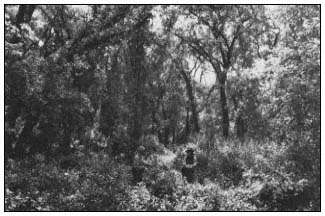
Figure 3.
Floodplain riparian system at Caswell State Park.
This area has been protected from disturbance
for several decades. (Photograph by R.E. Warner.)

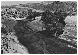
Figure 4.
Cantua Creek, a small perennial stream system in the Coast
Ranges. Note the heavy growth of sedges and the scattered
mature cottonwoods. (Photograph by R.E. Warner.)

ian system on the lower Stanislaus River, San Joaquin County; Kaweah River is a well-wooded, formerly grazed Sierra foothill stream near the town of Three Rivers, Tulare County; Cantua Creek is a heavily grazed, secondarily simplified system in the Coast Range foothills west of Fresno, Fresno County; and the San Joaquin River site is a vegetated levee on the floodplain near Stockton. Table 2 summarizes groundcover data for the four sites in terms of percent occurrence and mean height in decimeters, by groundcover-type.

Each site, as demonstrated here, had a unique set of groundcover characteristics reflecting its location, geophysical and hydrologic circumstances, land-use history, and present land-use patterns. Note, for example, the great difference in grass groundcover between Caswell (21.5%) and Cantua (70.6%) (table 2). Mean percent grass groundcover for all Central Valley sites combined was 41%; thus, Caswell was demonstrably below (19.5%) and Cantua well above (29.6%) the valley-wide average. Similarly, note the great disparity in forbs (non-grass herbs), where San Joaquin (25.0%) has over 16 times as many as Cantua (1.5%). The mean value for all Central Valley sites was 14%. Thus San Joaquin was well above the average value for forbs while Cantua was well below average. The high grass/low forb groundcover scores for Cantua reflect the long history of open-range grazing that particular riparian system has experienced. It also is linked to the reduced amount of tree canopy at that site, similarly the result of long-term open-range grazing. These figures can change very markedly over time for any site, depending upon overall land-use practices, and can be used as quantitative elements to monitor the systems, if desired. Information on canopy structure and floristics is presented below to further illustrate the high degree of intersite diversity.

Groundcover Floristics

Conspicuously absent from this portion of the inventory are data on the plant species comprising the groundcover. The decision was made during project design to preclude collecting locational and floristics data on the many groundcover species because of the limited time available both for developing the inventory procedures and for acquiring field data. Grasses, forbs, herbs, mosses, ferns, lichens, and other groundcover plant species are important components of riparian system structure and plant diversity, and ideally should be included in riparian inventory and monitoring programs. They present special problems of location and taxonomy because of the intense seasonality of growth and flowering. Where time and resources permit, their inclusion into riparian inventory design is recommended.

Shrubcover, Understory, and Canopy

Each of these vegetation strata are potential structural components of riparian vegetations. In this study, plants were considered "shrubs" if they had woody stems supporting leafy

vegetation above ground level, but were no taller than 6 m. "Canopy" was the leafy vegetation produced by trees, and "understory" was that (rare, as it turned out) vegetation layer below and in the shade of an over-arching canopy, residing between it and the underlying shrubcover stratum. Normally, each vegetation stratum should be treated individually, as each contributes separately to the morphological structure, floristics, and spatial patterning of a vegetation. For reasons of space in this paper, these three vegetative components are not analyzed separately. Table 3 summarizes, by plant species and relative frequency of occurrence, the patterns of shrubcover, understory, and canopy for all 51 Central Valley sites studied on the ground.

A total of 50 plant species was recorded for the entire Central Valley. This does not, of course, mean that this is the total number of riparian species in the Central Valley, as the total sample size and sampling procedures did not permit identification of rarer species. However, the table clearly demonstrates the relative frequency and abundance of those species which are of major structural and ecological significance for riparian systems within the study area. Some are detailed below.

Literature Cited

Anderson, B.W., and R.D. Ohmart. 1977. Vegetation structure and bird use in the lower Colorado River Valley. p. 23–24. In : R.R. Johnson and D.A. Jones (tech. coord.). Importance, preservation and management of riparian habitat: A symposium. [Tucson, Arizona, July 9, 1977.] USDA Forest Service GTR-RM-43, Rocky Mountain Forest and Range Experiment Station, Fort Collins, Colo. 217 p.
Bonner, K.G., L.D. Bowden, and R.R. Colwell. 1979. Riparian vegetation mapping and inventory design. (Draft.) Final report of work performed for the California Department of Fish and Game, Standard Agreement DFG-S-1729. Remote Sensing Research Program, Department of Forestry and Conservation, College of Natural Resources, University of California, Berkeley. 93 p.
California Department of Public Works. 1931(a). Sacramento Valley basin. Bull. No. 26, Division of Water Resources. California Department of Public Works, Sacramento.
California Department of Public Works. 1931(b). San Joaquin Valley basin. Bull. No. 29, Division of Water Resources. California Department of Public Works, Sacramento.
Carothers, S.W., R.R. Johnson, and S.W. Aitchison. 1974. Population structure and social organization of southwestern riparian birds. Amer. Zool. 14:97–108.
Akins, G.J., and C.Q. Jefferson. 1973. Coastal wetlands of Oregon. 159 p. Oregon Coastal Conservation and Development Commission, Florence, Oregon.
American Geological Institute. 1962. Dictionary of geological terms. 545 p. Anchor Press, Garden City, N.Y.
Austin, G.T., and W.G. Bradley. 1971. The avifauna of Clark County, Nevada. J. Ariz. Acad. Sci. 6(4):283–303.
Brown, D.E., C.H. Lowe, and C.P. Pase. 1979. A digitized classification system for the biotic communities of North America, with community (Series) and association examples for the Southwest. J. Ariz.-Nev. Acad. Sci. 14(Suppl. 1):1–16.
Brown, D.E., C.H. Lowe, and C.P. Pase. 1980. A digitized systematic classification for ecosystems with an illustrated summary of the natural vegetation of North America. USDA Forest Service GTR-RM-73, Rocky Mountain Forest and Range Experiment Station, Fort Collins, Colo. 93 p.
Campbell, C.J., and W. Green. 1968. Perpetual succession of stream-channel vegetation in a semiarid region. J. Ariz. Acad. Sci. 5:86–98.
Carothers, S.W. 1977. Importance, preservation, and management of riparian habitats: an overview. p. 2–4. In : R.R. Johnson and D.A. Jones (tech. coord.). Importance, preservation, and management of riparian habitat: a symposium. [Tuscon, Arizona, July 9, 1977.] USDA Forest Service GTR-RM-43, Rocky Mountain Forest and Range Experiment Station, Fort Collins, Colo. 217 p.
Carothers, S.W., and R.R. Johnson. 1975. Water management practices and their effects on nongame birds in range habitats. p. 210–222. In : Proceedings of the symposium on management of forest and range habitats for nongame birds. USDA Forest Service GTR-1, Washington, D.C.
Cowardin, L.M. 1978. Wetland classification in the United States. J. Forestry. 1978 (Oct.):666–668.
Cowardin. L.M., V. Carter, F.C. Golet, and E.T. LaRoe. 1979. Classification of wetlands and deepwater habitats of the United States. USDI Fish and Wildlife Service FWS/OBS79/31, Washington, D.C. 103 p.
Hanson, H.C. 1962. Dictionary of ecology. 382 p. Philosophical Library, New York, N.Y.
Hubbard. J.P. 1971. The summer birds of the Gila Valley, New Mexico. Nemouria (Occ. Pap. Del. Mus. Nat. Hist.) 2:1–35. Greenville, Del.
Johnson, R.R. 1978a. Foreword. p. ii. In : R.R. Johnson and J.F. McCormick (tech. coord.). Strategies for protection and management of floodplain wetlands and other riparian ecosystems: Proceedings of the symposium. [Callaway Gardens, Georgia, December 11–13, 1978]. USDA Forest Service GTR-WO-12, Washington, D.C. 410 p.
Johnson, R.R. 1978b. The lower Colorado River: a western system. p. 41–55. In : R.R. Johnson and J.F. McCormick (tech. coord.). Strategies for protection and management of floodplain wetlands and other riparian ecosystems: Proceedings of the symposium. [Callaway Gardens, Georgia, December 11–13, 1978]. USDA Forest Service GTR-WO-12, Washington, D.C. 410 p.
Johnson, R.R., and S.W. Carothers. 1982. Southwestern riparian habitats and recreation: interrelationships and impacts in the Southwest and Rocky Mountain region. Eisenhower Consortium Bull. 12, USDA Forest Service, Rocky Mountain Forest and Range Experiment Station, Fort Collins, Colo. 31 p.
Johnson, R.R., S.W. Carothers, and B.T. Brown. In press a. Perennial intermittent and ephmeral riparian habitats in the Southwest. J. Ariz.-Nev. Acad. Sci., Tempe, Ariz.
Johnson, R.R., S.W. Carothers, and N.H. Goldberg. In press b. Western riparian ecosystems: endangered natural communities. Burgess Publishing Company, Minneapolis, Minn.
Johnson, R.R., and L.T. Haight. 1983. Riparian problems and initiatives in the American Southwest: A regional perspective. In : R.E. Warner and K.M. Hendrix (ed.). California Riparian Systems. [University of California, Davis, September 17–19, 1981.] University of California Press, Berkeley.
Johnson, R.R., L.T. Haight, and J.M. Simpson. 1977. Endangered species vs. endangered habitats: a concept. p. 68–79. In : R.R. Johnson and D.A. Jones (tech. coord.). Importance, preservation, and management of riparian habitat: a symposium. [Tuscon, Arizona, July 9, 1977.] USDA Forest Service GTR-RM-43, Rocky Mountain Forest and Range Experiment Station, Fort Collins, Colo. 217 p.
Johnson, R.R., and D.A. Jones (tech. coord.). 1977. Importance, preservation and management of riparian habitat: a symposium. [Tuscon, Arizona, July 9, 1977.] USDA Forest Service GTR-RM-43, Rocky Mountain Forest and Range Experiment Station, Fort Collins, Colo. 217 p.
Johnson, R.R., and J.F. McCormick (tech. coord.). 1978. Strategies for the protection and management of floodplain wetlands and other riparian ecosystems: Proceedings of the symposium. [Callaway Gardens, Georgia, December 11–13, 1978]. USDA Forest Service GTR-WO-12, Washington, D.C. 410 p.
Langbein, W.B., and K.T. Iseri. 1960. General introduction and hydrologic definitions. USDI Geological Survey Water Sup. Pap. 1541-A. 29 p. US Government Printing Office, Washington, D.C.
Lowe, C.H. (ed.). 1964. The vertebrates of Arizona. 270 p. University of Arizona Press, Tucson.
McCormick, J.F. 1978. A summary of the National Riparian Symposium: A proposal for a national riparian program. p. 362–363. In : R.R. Johnson and J.F. McCormick (tech. coord.). Strategies for the protection and management of floodplain wetlands and other riparian ecosystems: Proceedings of the symposium. [Callaway Gardens, Georgia, December 11–13, 1978]. USDA Forest Service GTR-WO-12, Washington, D.C. 410 p.
Minckley, W.L., and D.E. Brown. 1982. Wetlands. In : D.E. Brown (ed.). Biotic communities of the American Southwest United States and Mexico. Desert Plants 4:223–341.
Oxford English Dictionary (Unabridged). 1979.
Random House Unabridged Dictionary. 1967.
Reed, P.B., Jr. In press. Differentiating between a classification system and a data base. Paper presented at "In-place Resource Inventories; principle and practice: a national workshop. [University of Maine, Arno, August 9–14, 1981]. USDA Forest Service.
Reid, G.K., and R.D. Wood. 1976. Ecology of inland waters and estuaries. 485 p. D. VanNostrand and Company, New York, N.Y.
Shelford, V.E. 1963. The ecology of North America. 610 p. University of Illinois Press, Urbana.
Swift, B.L., and J.J. Barclay. 1980. Status of riparian ecosystems in the United States. 29 p. USDI Fish and Wildlife Service, Kearneysville, W. Va. Unpublished manuscript presented at the 1980 American Water Resources Association National Conference, Minneapolis, Minn.
Thomas, J.W., C. Maser, and J.E. Rodiek. 1979. Riparian zones. p. 40–47. In : J.W. Thomas (tech. ed.). Wildlife habitats in managed forests: the Blue Mountains of Oregon and Washington. USDA Forest Service Agricultural Handbook No. 553, Washington, D.C. 512 p.
Warner, R.E. 1979. California riparian study program. 177 p. California Department of Fish and Game, Planning Branch, Sacramento.
Zimmerman, D.A. 1970. Birds of the Gila River Valley, New Mexico. Unpublished manuscript, Gila National Forest, Silver City. N.M.