
Regulatory Choices A Perspective on Developments in Energy Policy
EDITED BY
Richard J. Gilbert
Table of Contents
- ACKNOWLEDGMENTS
- ONE Introduction and Overview
- TWO Energy Utility Pricing and Customer Response The Recent Record in California
- THREE Issues in Public Utility Regulation
- FOUR The Value of Rate Reform in a Competitive Electric Power Market
- FIVE Natural Gas Distribution in California Regulation, Strategy, and Market Structure
- SIX Estimating Costs of Alternative Electric Power Sources for California
- SEVEN An Economic Evaluation of the Costs and Benefits of Diablo Canyon
- EIGHT Residential Energy Conservation Standards, Subsidies, and Public Programs
- NINE Wind Power in California A Case Study of Targeted Tax Subsidies
- TEN Concluding Remarks on the Making of Public Policy
- INDEX
ACKNOWLEDGMENTS
This book is the end result of a research program supported by the Universitywide Energy Research Group (UERG) of the University of California. We are indebted to the support made available by the University of California and to many of our colleagues who made this effort possible. Mike Lederer, Deputy Director of UERG, deserves the title of executive producer for this project. He helped organize meetings, communicate results, and iron out our differences. Mike thoroughly edited the final manuscript and made many important contributions. If our end product shows a semblance of order, it is in large measure a consequence of Mike's help.
Carl Blumstein, also of UERG, contributed his time and efforts to help keep our project on track. Carl worked with our able copyeditor, Suzanne Holt, and provided valuable advice to the team. Ed Kahn provided valuable comments during his visit to UERG. We are also grateful to Kermit Kubitz, Roger Noll, and Mason Willrich for their suggestions.
I can't give enough thanks to our UERG staff, Carol Kozlowski and Linda Dayce. Carol and Linda worked tirelessly to prepare working drafts and the final manuscript. They endured our many revisions. Their support and good humor were indispensable.
Finally, I have to thank my colleagues whose names appear in this book. Differences of opinion and methodology are inevitable and they are apparent in this book. I am happy to say that we saw through our differences and those that remain reflect the controversy and intellectual excitement of this field.
ONE
Introduction and Overview
Richard J. Gilbert
This book is an attempt to apply an economist's microscope to the process of public utility regulation. Long the bastion of the status quo, public utility regulation has felt the surge of deregulation proposals that have swept the country. Some of the most innovative and far-reaching programs of regulatory reform have originated in the state of California. In this volume we examine the results of this "new" regulation and consider some of the prospects for further reforms. Part I deals with issues in utility ratemaking. Perhaps the most basic principle of public utility economics is the desirability of prices that are as close as possible to marginal production costs.1 Marginal cost is the additional expenditure required to serve a small increase in demand. Economic principles dictate that the rate each customer should pay should be closely related to the marginal cost of serving that customer.
Traditional utility regulation is concerned with setting rates that just recover the cost of providing service. Rates for particular classes of service, such as residential and industrial, have responded to political pressures to favor one group over another. Often lost in this process is the value of utility rates as measures of the cost of meeting additional demand, i.e., the marginal cost of serving a customer.
Many factors complicate the calculation of marginal cost and its use as a bench mark for rate design. Marginal cost varies over time as utilities
respond to changing demand by altering the mix of production facilities. Marginal cost is also very sensitive to changes in the price of fuel or other factors of production. Making rates track marginal cost at every instant of time would be like tracking the tail of a dog. Even if it can be done, it is not clear that it is worth the effort.
Chapter 2 surveys a number of issues in utility rate design, focusing on the application of marginal cost principles and the difficulties that arise in trying to design and implement policies based upon them. In this chapter L. S. Friedman argues that utility rate design should deal with the complex circumstances that determine a consumer's demand for energy. Consumers might confuse the average cost of electricity with the marginal cost of an increase in consumption. The latter is the real cost to the consumer of a change in consumption, but the consumer might rely on the average bill as a signal of energy costs. By allowing for the idiosyncrasies of consumer behavior, regulators may be able to improve the efficiency of the electric power market. An example is energy-efficiency standards for residential appliances. In addition, if consumers rely on current prices as the main source of information about future economic conditions, there is a case for pricing at levels that are closer to long-run instead of short-run marginal costs. However, Friedman notes that these recommendations must be highly qualified. Although several studies indicate economic imperfections in residential energy decision-making, the regulatory record to date does not show much evidence that regulators are better able than consumers to predict future energy prices and to set rates that lead consumers to act in their own economic interests.
Chapter 3 reviews the role of utility regulation in sharing the risks of capital investment. A main economic function of regulation is to provide a stable financial environment that permits a utility to invest in large capital projects, while at the same time protecting consumers from the exercise of the utility's market power. But in this area, regulation may have succeeded too well. Regulatory policy in the period of the 1960s and early 1970s encouraged utilities to invest in projects that, in retrospect, exceeded the managerial resources of many companies (examples are the ill-fated Washington Public Power Supply System and Public Service of New Hampshire). The Public Utility Holding Act of 1935 discourages merger activity in this industry, as do regulatory policies that prevent stockholders from reaping the rewards of sharp management and from bearing the consequences of errors. In Chapter 3 I argue that the Public Utility Holding Act should be repealed or amended to encourage a restructuring of utility capital and allow utilities to better exploit managerial and technical expertise. In addition, regulatory policy should be changed to replace the "cost-plus" nature of rate-
of-return regulation with a system that compensates firms for superior performance.
Chapter 4 examines the potential gain from rate reform in the market for electric power. In California (and in many other states) residential customers pay rates that, relative to the marginal costs of service, are lower than the rates paid by commercial and industrial customers. In addition, California residential customers with moderate energy needs benefit from an "increasing block" rate structure, in which the marginal price of electricity increases with use.
This pattern of utility rates came about in response to both economic and political pressures. When increasing block rates were first mandated by California state law, the marginal price of electricity was high relative to historical average costs. Increasing block rates had an economic rationale because they raised the marginal price of electricity for most customers to a range that was closer to the anticipated long-run marginal cost of service. Since that time new capacity additions, increases in utility reserve margins, and lower fuel costs have sent marginal costs into a nosedive while the average cost of electricity production has soared. In this economic environment increasing block rates aggravate the spread between the marginal prices that customers face and the marginal costs of serving them. High prices tempt large industrial and commercial users to invest in alternative energy sources, sometimes at costs higher than the marginal cost of utility power. Such investment is termed "self-generation" when a customer generates electricity for his own use. Self-generation is an example of the more general phenomenon of "bypass," which occurs whenever a customer replaces utility-generated electricity with an alternative source of supply. The resulting losses in economic efficiency are large. John Henly and I estimate that inefficient pricing of electric power costs California alone about one billion dollars per year. Chapter 4 considers various options to improve the economic efficiency of electricity pricing. Pricing schedules whose effects are limited to rearranging revenue burdens between customer classes or over time have, by themselves, only a modest potential for increased efficiency. The reason is that they do little to close the large gap between price and marginal cost. The use of two-part tariffs or declining block rates can allow prices to move closer to marginal production costs, but the distributional effects in the residential class are unpleasant and the potential efficiency gains for industrial and commercial consumers are constrained by their substitution possibilities. The largest scope for improvement lies in a coordinated approach to rate design that combines a reallocation of revenues across customers with a reallocation of revenues across time. Taking advantage of the likelihood that marginal costs will increase relative to average costs in the future allows regulators to borrow from the future
and narrow the present cost gap. This permits efficiency gains from marginal-cost pricing with smaller distributional impacts.
Chapter 5 is a broad look at regulatory trends in the natural gas distribution industry. Partial deregulation of natural gas wellhead prices began in 1985 according to the provisions of the Natural Gas Policy Act of 1978. The sudden increase in prices predicted by many opponents of deregulation did not materialize, and the only dramatic price movements were in the downward direction as markets responded to a surplus of natural gas. Russo and Teece refer to a "take-or-pay crisis," which resulted when natural gas distribution companies entered into firm contracts for the delivery of gas supplies without a guaranteed demand. As the gas markets softened these companies were caught in a squeeze, with mounting supplies and shrinking demand.
A major development in the natural gas industry is the emergence of contract carriage, in which end users contract directly with gas producers and pay the distribution company only for the cost of moving the gas. This contrasts with prevailing practice in which distribution companies purchase gas supplies for resale. Contract carriage is a move toward a deregulated gas market, in that consumers and producers can search freely to make the most attractive deals. Russo and Teece believe that some form of voluntary (or perhaps mandatory) contract carriage should accompany the decontrol of wellhead prices to insure that the benefits of decontrol are not captured by pipelines.
Russo and Teece point to evidence of low market concentration in natural gas production and conclude that "on strictly efficiency terms, the argument for continued regulation of any gas reserves is weak." The picture is less clear in natural gas distribution. Although many large markets are served by several pipelines, and most large customers have alternative sources of supplies, capacity limitations and the immobility of distribution capital may allow exercise of market power in specific situations.
Rate design in the natural gas market, as in electricity, illustrates the interplay of politics and economics that characterizes public utility regulation. Political pressures have favored residential consumers in recent years, while the ability of industrial and large commercial customers to bypass the utility have favored rate reductions for these classes. A novel twist in public utility regulation is the recent designation by the California Public Utilities Commission of "core" and "non-core" customer classes, which receive different treatment, not only for the pricing of gas, but also with respect to procurement of new supplies. Although this regulatory innovation can (and will) be criticized for its unequal treatment of different' customer classes, it is nonetheless a step forward because it recognizes the importance of narrowing the gap between price and the
marginal cost of service for those customers whose demands are particularly sensitive to price. In addition to the economic distortions from prices that diverge from marginal costs, Russo and Teece argue that regulation has contributed to inefficiency by failing to provide utilities with sufficient incentives to contain their costs.
Part II of the book moves from problems of rate design to problems of energy supply. A survey of cost estimates for alternative energy sources is the subject of Chapter 6 by Mead and Denning. In addition to surveying studies of private (direct) energy costs, they also attempt to include estimates of social costs (the total of direct costs and health and environmental impacts). The energy sources they examine include coal, oil, natural gas, nuclear, wind, solar, biomass, and imports of surplus power from the Northwest and Southwest.
Mead and Denning expect economic growth and lower oil and gas prices (relative to the early 1980s prices of about $32-34/bbl) to cause an increase in electricity demand that will require new reserve additions in the state of California within a decade. They point out that although imports from the Southwest and Pacific Northwest (primarily surplus hydropower) can fill short-term needs, increasing electricity demand in the West will soon eliminate that surplus. Mead and Denning are bullish on the potential for thermal power, particularly nuclear and coal, to meet the electricity needs of the West. They find little evidence to support the view that unconventional sources—solar, biomass, and wind— can provide the large amounts of electric power that will be demanded in the future at social costs that are competitive with coal, nuclear and imports of surplus power. They attribute much of the disappointment with the performance of nuclear power to excessive costs imposed by intervenors and to unnecessarily burdensome regulations, although this conclusion has to be considered in light of the managerial problems that have plagued the industry. Pointing to the low construction costs achieved in other countries and by those U.S. utilities whose construction programs have proceeded smoothly, they argue that nuclear power can be an economic source of electric power.
Chapter 7 is a case study of the Diablo Canyon nuclear power plant, built by the Pacific Gas and Electric Company. The Diablo Canyon plant embodies much of the frustration that has accompanied the U.S. commercial nuclear program. The plant took more than 15 years to complete. Originally forecast to cost about $450 million, the book cost of the completed plant was $5.7 billion. In 1985 dollars, and including allowances for the opportunity cost of capital, the plant cost almost seven billion dollars.
Although Diablo Canyon may never produce benefits that cover its costs, Cox and I claim that, on the basis of information known at the
time, proceeding with Diablo Canyon in the decade of the 1980s was economically justified even if the large cost overruns could have been correctly anticipated. In the late 1970s and early 1980s, most forecasters projected that the value of oil and gas that would be displaced by the plant would exceed the plant's cost, even including eventual overruns. Actual and forecast oil and gas prices fell in the last years of the Diablo Canyon project, but by that time sufficient capital had been sunk into the plant that it made economic sense to continue with the construction program. Thus, based on commonly accepted forecasts and the history of expenditures, the Diablo Canyon nuclear power plant (and many other utility projects in the U.S. that shared a similar history) was an appropriate investment decision. Of course this analysis does not consider whether Doable Canyon's cost overruns were avoidable, or whether other investment strategies could have replaced Doable Canyon at lower cost or lower risk.
Part III of our monograph takes a look at the results of programs designed to subsidize particular energy projects. In Parts I and II, the discussion focused on the process of utility regulation, the principles of rate design, and on the economic evaluation of energy sources. The topics in this section differ in that they deal with the effects of market intervention that is targeted to the promotion of a particular course of action.
Our objective in this section is to review the results of selected "target" subsidy programs with attention to the magnitude of the results and their economic costs. We do this for the case of residential energy conservation programs and wind power. In Chapter 8 Quigley takes a hard look at the record of programs to encourage residential energy conservation in California. Quigley finds a very wide variation in the economic effectiveness of different conservation programs. At the top of the list is a utility-provided service to turn pilot lights on and off, which cost less than a dollar for each barrel of oil (or natural gas measured on an oil-equivalent energy basis) saved by the program. But other programs were not nearly so cost-effective. Solar financing programs absorbed about $50 for every barrel saved, and many other residential energy conservation programs were in the $20-$40 range.
Quigley's results show that the potential exists for cost-effective subsidies in the area of energy conservation, but it is crucial to monitor the results of these programs carefully and winnow out those that absorb more in subsidies than they deliver in energy savings. Moreover, Quigley shows that in many cases the burdens of these programs fall disproportionally on the poor. Federal and state energy conservation tax credits were claimed predominantly by people in higher income brackets, often for the solar heating of pools and hot tubs before these applications were
curtailed. The costs of these programs were borne by all taxpayers, while the benefits (as measured by both tax credits and energy investments) were enjoyed by those with higher incomes. Energy conservation programs can work, and sometimes with spectacular success, but they are not a free lunch.
Compared to residential energy conservation, it takes a Don Quixote to find inspiration from the economic performance of subsidies for wind power. The development of wind power in California was stimulated by the availability of federal and state tax credits and legislation promoting favorable rates for the purchase of non-utility power. The results were dramatic. Over a space of five years, more than a billion dollars was spent on wind power in California and installed capacity grew to more than 1,200 MW. The vehicle for nearly all of this growth was the limited partnership, which enabled individual investors to reap the benefits of the tax provisions.
The subsidies for wind power succeeded in establishing a source of supply, but at a high cost. Windmills currently operate in the state on a commercial basis. These are small to moderate-sized machines with short construction lead times and relatively unsophisticated design. The federally sponsored research and development program for wind power concentrated on very large machines. Although these may prove economic in the future, in contrast to the private partnerships, the federal program has yet to demonstrate a commercially useful machine.
Although the California machines are in commercial use, their profitability depends on the existence of tax subsidies and long-term electricity price guarantees. In Chapter 9 Blumstein, Cox and I show that the California wind power program produced a net loss of about $2 billion, shared by California ratepayers and California and federal taxpayers (as well as by some investors who failed to break even, despite large tax write-offs). The subsidies succeeded in promoting development of a commercial industry, and substantial improvements in costs and reliability have been achieved since the subsidies were first offered. But despite this progress, we conclude that the benefits were not worth the costs. At current energy prices the windmill industry is not commercially viable in the absence of continued state and federal subsidies. Although it is useful to know that a windmill industry can exist and supply electricity to the grid, this information could have been obtained at much lower cost. Earlier termination of tax subsidies could have succeeded in accumulating adequate information about the capabilities of wind power with considerably less investment.
What conclusions wind their way through this book? One clear message is that even regulated industries are not immune from the forces of competition. Regulators are not free to design rate structures and
incentive programs without regard for the economic conditions of the market. Technological, political and economic changes in the industry have made energy industries more responsive to competition. Scale economies have diminished somewhat, making competition easier. The Public Utility Regulatory Policies Act of 1978 mandates utilities to contract with independent sources of supply, and is a chink in the regulatory armor.
Another conclusion is that regulators have always had a hard time outguessing the market and will continue to do so. Innovative regulatory programs have been a mixed bag. The record of energy subsidies targeted at specific industries, such as the renewable energy tax credits, has been dismal. The wind energy program in California was an elaborate structure that pumped dollars from ratepayers and federal and state treasuries into the pockets of general partners and underwriters, in the process creating a new energy industry with only marginal viability in the absence of continued subsidies. In contrast, some conservation programs have produced significant economic benefits. The most successful programs appear to be those that deal with a lack of consumer information, such as appliance efficiency labeling. Programs designed to subsidize new technologies have fared much worse.
Our consensus view is that regulatory policy should try harder to imitate the function of the marketplace. Current price structures in electric power and natural gas bear too little resemblance to marginal-cost pricing, or even to approximations of marginal-cost pricing that satisfy the constraint of meeting revenue requirements. Innovative rate design, such as nonlinear and interruptible prices, can go a long way toward improving the way in which energy is used and can mitigate the cost of inefficient "bypass" of regulated services.
We have largely ignored the question of whether regulation should be abandoned. Although this is an intriguing prospect, we believe that this question is not critical to our energy future, because regulation must in any case respond to the forces of competition that are developing in this industry. Independent power production and bypass of traditionally regulated utility services will exist in the electric power industry whether or not electric power generation is deregulated. Competition for natural gas supplies and for alternative fuels will exist independent of regulation, although measures such as contract carriage can greatly increase the scope for competition.
Another area that this book ignores is the interaction between environmental and energy policies. Although Mead and Denning estimate some of the costs of environmental damage from coal and nuclear supply systems, this is a limited effort. Moreover, societal objectives such as the use of best available emission control technologies mean that the im-
plementation of pollution abatement measures need not have a direct relation to the costs that energy technologies impose on the environment. With respect to environmental impacts, an analytical approach that attempts to define appropriate pollution control measures based on the cost of environmental damage from energy technologies need not result in recommendations that are agreeable to the voting public. Yet public sentiment about environmental consequences can have major impacts on the evolution of energy supply and demand. For example, even with a full accounting of the economic costs of environmental hazards, it is unlikely that in the near term solar and wind power could be justified as economic sources of supply relative to fossil fuels with pollution abatement technology. Yet this need not interfere with a public determination to promote solar and wind power as alternative sources of supply.
Regulators have become more responsive to changes in energy markets, but their performance shows little cause to conclude that regulation is "better" today than it has been in the past. Economists' skepticism of the workings of regulated markets remains valid. Political pressures offer too many opportunities to interfere with economic efficiency. There is as yet little evidence that regulators act as if they are fully aware of the limits of their information about the markets they attempt to control. As competition increases in the energy industries, as we expect it will, we wonder whether regulators will adapt to competitive forces or attempt to further isolate the industry from change. The challenge to regulation is how to cope with these emerging forces while attempting to fulfill its traditional economic role of protecting consumers from abuses of market power.
TWO
Energy Utility Pricing and Customer Response The Recent Record in California
Lee S. Friedman
I. INTRODUCTION
This chapter surveys a variety of ideas and policy reforms concerning consumer demand for utility-provided energy. The focus is primarily on pricing policies and how they affect demand. Evaluative discussion relies on traditional economic criteria. However, in the discussion special analytic emphasis is placed on the importance of understanding actual consumer responses to complex decision problems and political and organizational constraints faced by policy makers. Data and examples are drawn largely from electric utilities in California, with emphasis on the regulatory role of the California Public Utilities Commission (CPUC).
The chapter is organized as follows. First, I briefly review some general aspects of consumer demand for energy, the institutional setting for its regulation, and the economic criteria used to evaluate pricing policies. Then I describe the process of rate setting in California and the actors involved. The description emphasizes the limited attention given to economic reasoning in the regulatory process. I conclude that the nature of this process leaves considerable room for the acceptance of economic analysis, provided that its implementation is not too complex.
I then examine recent policies for rate structure in California and proposals for their reform. These policies include the method of reve-
nue allocation and the use of charges for maximum instantaneous demand within a month, time-of-use (TOU) prices, and prices that vary with service reliability. In each case, the complexity of the customer's decision problem is considered as a factor in evaluating proposed reforms. A final section provides a summary and conclusions.
II. PRICING UTILITY-SUPPLIED ENERGY: THE INSTITUTIONAL SETTING AND ECONOMIC CRITERIA
There is a great public interest in understanding and regulating consumer demands for energy resources. In this age of heightened environmental sensitivity, it is easy to see the reason for this interest. The demands of consumers for electricity and natural gas influence the rate at which we use up exhaustible resources, such as oil (to fuel power plants) and wilderness areas with rivers (to build new sources of hydroelectric power). They influence our perceived needs for using controversial technologies, such as nuclear generating plants. Energy demands are important because of their primary functions: their uses for basic heating and cooling influence our health and our comfort at home and at work, and their uses within firms influence the cost and composition of goods and services produced in the economy and thus our overall economic well-being. If the public interest is to be served, it is important that our energy policies be as rational as possible.
To understand the policy issues that arise in energy pricing, one must have a sense of the institutional settings in which policies are formulated, debated, and implemented. Energy utilities in the United States virtually always operate under one of two types of institutional arrangement: (1) a privately owned company the retail rates of which are regulated by a public utilities commission (PUC) or (2) a publicly owned and operated enterprise. In either case, the public sector has direct and continual responsibilities for the setting of utility prices. The analysis of rate design issues I shall be discussing applies generally to both institutional arrangements, because the public sector powers and responsibilities are similar.1
The primary reason for the particular institutional arrangements that characterize energy provision is that the technical features of the energy distribution system make it a natural monopoly. It is not sensible to have more than one set of electric wires or natural gas pipes distributing
energy to particular physical locations.2 However, if there is only one private profit-seeking supplier to serve customers in the area, with neither competition from alternative suppliers nor regulation by the public sector, what forces would act to prevent monopolistic price gouging and service of poor quality or inadequate quantity? Thus energy utilities have historically been regulated or operated by the public sector, as have providers of local telephone service and water.
Traditionally, public sector officials have emphasized the need for equitable prices. Various conceptions of equity may underlie different aspects of ratemaking. For example, virtually every state PUC limits the total revenues collected by a utility to consist of operating costs plus a normal profit (a "fair" rate of return on capital). In recent years a small number of states have adopted explicit policies to ensure that some minimal level of energy is available at a subsidized rate to some or all residential customers. State PUCs also have responsibility for the efficiency with which scarce energy resources are used, and in recent years attention to this aspect of energy regulation has been growing.
When economists have analyzed local power provision, they have always used one key principle in their pricing recommendations: prices should be based on marginal opportunity costs. The opportunity cost refers to the value of the resources used to provide a service in their best alternative uses. If a price is set equal to the marginal opportunity cost of supplying a service, then, in effect, every potential consumer is encouraged to consider whether the benefits of additional consumption are greater or less than the costs in terms of foregone benefits from the best alternative use. If all customers perceive this and respond in a fully knowledgeable way, they will only consume those quantities for which the benefits outweigh the costs. This will result in the allocation of resources to their most highly valued uses; such an allocation is called efficient .
In fact, it is much simpler to advocate the use of theoretical principles than it is to achieve their implementation. Important real-world complexities, which theory often assumes away, must be faced. Thus perhaps it is not surprising that in the United States today only a handful of state PUCs (such as those in California, Oregon, New York, and Wisconsin) have embraced marginal-cost-based pricing principles. We shall use California as a case study of the progress made and problems encountered.
The CPUC first made explicit reference to marginal costs in rate design in 1979 (Parry, 1984). In its decisions it has indicated a rationale for using marginal costs virtually identical to the social objectives stated above: "The result of basing rates on marginal costs is that . . . each consumer pays the resource cost . . . Conservation is achieved since con-
sumption is made only when the benefits of consumption are greater than or equal to the cost . . . Efficiency is achieved since the least-cost combination of resources neither overuses the good nor underuses the good . . . Finally equity is achieved since no customer underpays relative to the resource cost" (California Public Utilities Commission, 1980, p. 10).
These laudable goals have been subservient to the objective of total cost recovery in utility ratemaking. The CPUC did not intend to set consumer prices equal to the marginal cost of providing utility service to the customer. Rather, the CPUC designed a formula using marginal-cost estimates to allocate the total cost of utility services to different customers such that each customer pays a rate that is a multiple of the marginal cost of serving that customer, with the same multiple for every customer. This is known as "equal-percentage of marginal cost" (EPMC) ratemaking. When the average cost of service differs from the customer's marginal cost, EPMC rates also differ from the marginal cost of service.
Notwithstanding the fact that EPMC ratemaking is only a partial move toward the principle of setting rates equal to marginal cost, progress in this direction has been impeded by other considerations. In general rate cases involving the Pacific Gas and Electric Company (PG&E) (1984) and the Southern California Edison Company (SCE) (1985), the CPUC chose to weight the revenue allocation among customer classes (residential, commercial, industrial) by only 5% based on marginal-cost considerations (EPMC) and 95% based on historical allocations.3 In other areas as well, the CPUC approves rates that depart significantly from those based on marginal costs. What is preventing, or retarding, more extensive use of marginal-cost principles? I shall consider and illustrate this shortly by examining several of the rate design questions at issue in a CPUC general rate case.
Most theoretical studies assume only a few prices to be set. But in actual practice utilities sell a large number of services and must set a price for each. For example, SCE has 49 different rate schedules for electricity sales (varying by the type of customer and service provided), each with between three and eight price components. Thus the CPUC must set hundreds of prices for just this one utility. Other utilities sell both electricity and natural gas and have even more rate schedules. The entire set of utility prices is referred to as the rate structure. Each component of the rate structure must be determined so that the revenues raised overall lead to the allowed profits. This complexity complicates considerably the
price-setting process. To consider the use of marginal-cost principles to determine the rate structure, it is useful to review its components.
Energy prices are set separately for the major classes of energy customers: residential, commercial, and industrial. Within any class of customers, price may vary by season and by time of day (e.g., peak load pricing), by the quantity purchased (e.g., connection charges, baseline or lifeline tier quantities), by the instantaneous speed or flow of delivery of the quantity (demand or maximum kilowatt charges), and by the quality in terms of reliability of the service purchased (interruptible contracts or direct load management services). Thus many rate schedules apply within a customer class, depending on the specific type of service a particular customer receives. A question of equity that typically arises in regulatory proceedings and constrains the prices in specific schedules concerns the proportion of total revenue that is raised from each major customer group; this is referred to as the class allocation issue.
Marginal-cost principles can be used to guide pricing of each component of the rate structure. The key question is whether each customer perceives the appropriate price for marginal changes in his consumption. Because the actual marginal cost varies substantially, depending on such factors as the time the service is demanded or the reliability of the service promised, the presumption is that the rate schedule should reflect these variations. Several of the ideas discussed in the literature, such as peak load pricing (also called time-of-day [TOD] and time-of-use [TOU] pricing) and interruptible contracts, have been tried as experiments or are used to a limited extent. However, many of these ideas have not received the widespread acceptance originally hoped for by their proponents. I shall consider the obstacles to their fuller implementation.
The next section reviews the actors involved in California rate setting and the process used to determine rates. Such review helps identify Political forces and organizational capabilities that constrain the use of marginal-cost pricing principles to achieve equity and efficiency objectives.
III. THE PRACTICE OF ENERGY UTILITY POLICY MAKING IN CALIFORNIA
In most respects, the institutional structure for regulating power utilities in California is similar to that used in other states. The CPUC is responsible for regulating the rates charged by private utility companies to their customers. Unlike most other states, California has a separate body, the California Energy Commission (CEC), which has regulatory
authority over utility requests to add new power sources. Because this chapter focuses on the rate-setting process, I will concentrate on the CPUC.
Every three years, each private utility initiates a general rate case.4 The utility requests authorization from the CPUC to charge particular rates, and the requests are analyzed and considered in a quasi-judicial process that takes about 14 months. Between general rate cases, rate adjustments are allowed through frequent "offset" rate proceedings. Offset proceedings are intended to adjust rates and revenues in response to changes in a utility's costs that are beyond management control. These costs are principally for fuel, and changes are largely based on the application of preexisting fuel adjustment clauses. Offset cases do not generally result in major policy changes.
The main issues of rate design are considered in the general rate cases. These cases have three stages: analysis, hearings, and decision making.5 CPUC staff analysis begins when the utility files a Notice of Intent to apply for rate changes, along with draft versions of its supporting testimony. Individual staff members from the CPUC Rate Design Branch are appointed to analyze the utility's rate structure proposal, and the commission selects one of its five members to oversee the case and appoints an administrative law judge to conduct the hearings.
About two months after the Notice of Intent is filed, the utility formally files its rate change application and submits final versions of its supporting arguments. The CPUC staff then has about three months to analyze the request and prepare its response and rate change proposals. Then the hearings begin. Testimony is given, with all parties (utilities, CPUC staff, and interest groups) represented by lawyers who can cross-examine witnesses. The hearings themselves usually last four or five months, and the presiding administrative law judge issues a draft decision about two months after the hearings are concluded.
The final stage of decision making begins with the issuance of the draft decision. The draft is circulated to the commissioners and senior staff, and within the next month oral arguments are formally presented to them by the parties to the case. Then the informal process of building consensus among the commissioners for an amended decision occurs, and the final decision is usually issued about two months after the start of this stage.
Substantively, each case proceeds in the same way. First, the utility's revenue requirement and marginal costs are determined. Second, the
commission comes to a broad decision about how to allocate that revenue among customer classes. Finally, actual rates within classes are set to raise the allotted revenue. However, a closer look at the process reveals important constraints not seen by considerations of substance alone. The logic in decision making is strongly influenced by the CPUC organizational routines, as well as the backgrounds of the individuals from the CPUC involved in the case.
About 20 staff members comprise the Rate Design Branch, with about two-thirds working on electricity issues and the rest working on natural gas. By training, roughly half have engineering backgrounds with a few economists, statisticians, business administrators and others comprising the balance. In making recommendations, the staff usually follows precedent from past cases. There are several important reasons for this. It eases the staffs heavy work load. Because the administrative law judges and the commissioners strongly attend to precedent in their reviews, following precedent is most likely to be acceptable to them. Acceptability is itself important in CPUC evaluation of the work of the Rate Design Branch. In addition, following precedent will result in fewer requests for additional work in the later stages of a rate case.
Another reason for often following precedent is that the staff typically lack the information necessary to apply innovative designs, such as those based on recent theoretical work in economics utilizing marginal-cost principles. Most of the Rate Design staff are unfamiliar with theoretical concepts such as optimal nonlinear pricing.6 The few economists on the staff have never attempted to apply any of the more sophisticated concepts from welfare economics to a specific electric rate design.
Furthermore, even if the staff were more inclined to apply such ideas, it does not generally have the necessary empirical information. For example, these ideas usually require knowledge of price responsiveness of the specific consumers affected by the design. But the Rate Design Branch only has a fixed sales estimate as input with which to work. The latter implies the false assumption of zero price responsiveness, but it has the great virtue Of simplicity and easy availability. These reasons explain why the Rate Design Branch usually follows precedent, although there are exceptions.7
The next organizational layer, the administrative law judges, adhere even more strongly to precedent. Most of the administrative law judges are lawyers, although some are engineers. Lawyers are, of course, highly
trained to attend to precedent. Furthermore, because these individuals are generalists who must deal with all aspects of rate cases, they are less familiar with the details of analytic methodologies applied to specific issues in a case. They are more comfortable checking arguments for consistency with prior decisions than making decisions on methodological grounds, such as those involving sophisticated economic reasoning.
In the final decision-making phase of the case, the role of the commissioners themselves takes on a great importance. The commissioners are not elected officials but are appointed by the governor for six-year terms. They rarely come to the job with experience in public utility regulation or knowledge of economics, and they are almost never reappointed. They generally see their role as one of avoiding "unfair" rate design. They check the rate design by eyeballing tables of numbers reflecting class allocations and residential rates. The underlying rationales for these numbers are not too important to them; significant departures from the outcomes of the current rate structure are. They demand repeated iterations of the numbers to see the effect of certain changes.
Because the commission often makes none of the major substantive decisions in the case until the final weeks, myriad frantic recalculations are typically necessary as the commission tries to reconcile modifications to one part with their implications elsewhere. For example, commissioners often do not decide the total revenue requirement until the last minute, which requires a revised class allocation decision and then recalculation of all specific components of the rate design. Thus the latter must be easily and quickly alterable to meet the overall requirement.
Naturally the utility being regulated fights hard for its positions throughout this process. However, the offset policies mentioned earlier have the effect of reducing the utility's stake in rate design. In particular, the energy rate adjustment mechanism (ERAM) insulates the utility on the revenue side, and the energy cost adjustment clause (ECAC) insulates it against changes in fuel costs. Both mechanisms provide for adjustments in the per-kilowatthour rates to ensure the collection of the forecasted (and CPUC approved) total revenues as well as to adjust for any differences between forecasted and actual fuel costs.
Except for administrative and other nonfuel operating costs, these clauses guarantee the dollar return to the utility specified in the general rate case. Thus unanticipated revenue and fuel cost effects of specific changes in the rate design (e.g., increased use of TOU rates) are eliminated by the adjustments. Although these clauses mitigate utility concern over rate design changes, they do not eliminate that concern. The utilities still prefer not to change the design if they think the change will confuse customers and create complaints. However, the clauses minimize utility opposition to rate design changes and thus enhance
the ability of the CPUC to experiment with marginal-cost-based pricing principles.8
To sum up this discussion, the process of deciding a general rate case reveals important constraints not seen by considerations of the substance alone. The economist interested in the increased use of marginal-cost-based principles must keep several ideas in mind. To increase chances for adoption, four characteristics are desirable for any new method of rate design. One is that it should be simple to calculate and should require only information that is already available or easily obtainable. Two is that it should be simple to explain to noneconomists, particularly the extent to which it utilizes principles acknowledged in prior decisions (and thus can be seen to have precedent). Three is that its distributional effects on consumers (particularly across recognized classes of consumers) should be minimal. Four, it should be easily understood by consumers. This last point is given more extended discussion in the following section.
IV. CONSUMER DEMAND FOR UTILITY-SUPPLIED ENERGY
Customer demands for utility-supplied energy are called derived demands: customers (whether residential, commercial, or industrial) are generally interested not in the energy per se, but in the services that use energy (e.g., lighting, heating, cooling). That is, the customers' demands for energy are derived from their demands for energy-using services. Many factors influence the derived demands for energy. It is useful to divide these factors into two broad categories: exogenous factors, which individual customers do not control, primarily technology and prices, and customer decision making in light of the exogenous factors.
The exogenous factors determine the options customers face for obtaining the (energy-using) services they seek. For example, the energy demanded by customers for the purpose of cooling a building depends on how much energy is used by the various air conditioners available on the market, as well as the availability and attributes of such alternatives
as thermal coating of windows or other insulating measures. The climate is another important exogenous factor. For buildings that already exist, the climate is determined by location. If constructing a new building, however, a customer may choose from among a variety of climates by deciding on a location.
Customer choice from among the available options depends on knowledge, preferences, and budget constraints.9 Knowledge refers to the customer's understanding of the various attributes of each alternative. For example, does the customer know how much energy a particular air conditioner will consume when operated, and does the customer know how much this energy will cost over the life of the air conditioner? Does the customer know how to translate future costs into present-value terms? Does the customer know about alternatives, such as thermal coated windows? Does the customer know how energy costs are affected by building or plant location in a hot region or a moderate one, even within a metropolitan area near a windy shore or a sheltered site inland? When making choices, some customers may have much more information than others faced with comparable choices and may use it more effectively.
In light of the customer's actual knowledge, choice still depends on the customer's preferences and budget constraints. To continue with the cooling example, the customer may have limited space for an air conditioner and therefore may seek a relatively compact one. Or a customer may seek an air conditioner that is unusually quiet. The residential customer may know about thermal window coatings but may not like their aesthetic effects. The industrial customer may know how much greater energy costs are in a southern location, but the quality of the available work force may be more important. Finally, the customer must reconcile preferences with economic means. Not everyone can afford a deluxe model air conditioner, and the purchase choice will reflect the customer's budget constraint.
These examples suggest the following points. We know from basic economics that energy prices are factors in customer decisions about how much energy to demand. However, in many cases prices may be minor factors compared with other attributes of the energy-using services customers seek. In making their decisions, fully informed consumers may consider extensively the consequences of energy prices.
Neverthless, in these cases, other factors may matter much more. In addition, many other customers may-perceive only dimly at best the consequences of energy prices for their decisions. In these latter cases, the effects of energy prices may be more difficult to analyze.
Public policy can affect the demand for utility-supplied energy through the use of diverse instruments. Prices can be lowered or raised to encourage or discourage the purchase of particular goods or services. Regulatory restrictions can be used to limit the range of options available to the consumer. Educational efforts can be undertaken to alter consumer choices from the available options. These actions can affect customer decisions directly, as well as indirectly, by causing changes in the available technologies for energy-using services.
Much of the rationale for policies involving regulatory restrictions and educational efforts depends on the assumed existence of important imperfections in the consumer decision-making process. To the extent that these imperfections are present, they may also affect pricing recommendations. Let us consider as an example technological regulations. These are restrictions that limit the choice of options available to consumers. Energy efficiency standards for refrigerators or required conservation measures in new homes and buildings affect demand by restricting the available options for energy-using appliances and structures. That is, these regulations are choice restrictions because they ban the sale of products (refrigerators and new homes) that do not meet the standards.
What is the rationale for such standards? Obviously the regulators must think that without the regulations too many refrigerators of the energy-hogging type are bought and too few conservation measures are installed in buildings. Do the regulators have different objectives than the consumers? According to the reports of the CEC, this is not the reason for such regulations in California. Rather, the CEC relies on the idea that many consumers will not be aware of the energy-cost implications of purchasing unregulated appliances or buildings and thus not act in their own best interests.10 If consumers only lack information, why not solve the problem through educational efforts rather than regulations? To this idea the commission responds by citing the difficulty and great expense of educating consumers and states "there are cases where it costs less to install measures for free than to provide information to consumers" (California Energy Commission 1983, p. 126).
Based on the studies available, the CEC appears to be on solid ground in its claim that energy consumers often do not act in their own best interests. According to evidence summarized by Stern, "people tend to overestimate the amounts of energy used by . . . technologies that must be activated each time they are used. Thus people overestimate energy use by televisions and lights and underestimate energy use by furnaces and water heaters . . . to save energy they will do more light dousing and less furnace retrofitting than is in their economic self-interest" (Stern, 1986, p. 205).
Furthermore, there is often little or no effect of providing information to consumers in the hope of inducing them to act in their own self-interest. Numerous factors explain this disappointing result. First, the information may be ignored if it is only relevant to a calculation the consumer does not know how to make. In a study of disaster insurance purchases, Kunreuther (1976) found many consumers who had no notion of expected-value calculations and thus no response to information about damage probabilities. With respect to energy consumption, consumers who have no notion of present-value calculations may ignore information about future energy prices.
Second, the form of the information matters a great deal. In one study, consumers receiving a carefully designed package of information cut energy use in response to TOU energy rates by 16% compared with a control group receiving the sponsoring utility company's standard information package (Heberlein and Baumgartner, 1985; cited in Stern, 1986, pp. 205-206). In another study, the best-designed information package increased the average efficiency of a household's choice to 51% from the 43% based on the standard utility-provided package; this example illustrates that even the best information efforts still result in large numbers of consumers making choices substantially worse than their optimal ones (Magat, Payne, and Brucato, 1986).11
Finally, the source of the information, particularly its trustworthiness, also matters to consumers. Two groups of energy consumers in New York State were sent conservation brochures that were identical except for the letterhead. The group receiving the brochure with the letterhead of the New York State Public Service Commission cut energy by 7% in the following month, compared with no reduction from the group receiving the brochure with the letterhead of Consolidated Edison. In another study, a county government with no energy expertise was five times as effective as an energy company in enrolling participants in the same home retrofit program offered at no cost to participants. In both cases, the difference was attributed to the differential trust consumers
had for the respective information sources (Craig and McCann, 1979; Miller and Ford, 1985; both discussed in Stern, 1986, p. 206). These studies also help explain why consumers often rely on the advice of non-expert friends while ignoring the advice of experts.
One of the missing pieces of information to many consumers may be the price of energy.12 To continue with the example of an air conditioner purchase, a customer should know not only current but future energy prices. That is, it is not enough to know how much electricity the air conditioner will use, but how much will be charged for that electricity, which depends on the price of electricity over the life of the air conditioner.
Figure 2.1 illustrates in one simple way why prices may be difficult to perceive. Imagine the following scenario, which is like the position of electric utilities with excess capacity in the late 1970s and early 1980s. Let De be the electricity demand originally expected by planners,13 and let the long-run marginal cost per unit including capacity be Q E These parameters lead planners to provide a capacity of Q C , where the demand and long-run marginal-cost lines intersect. However, actual demand turns out to be D A and if price P E were charged, only Q A units would be demanded and there would be much unused capacity in the system. Therefore price is set in the short run at P A , which makes the actual demand fully utilize the available capacity.14
In this scenario consumers are currently facing a price of P A per unit of electricity. However, suppose planners expect (more reliably this time) system demand to grow over the next few years to D F . Then, the utility will have to add new capacity (to Q F ) and in the future charge price P E .15 The question is, if you are the consumer deciding on an air conditioner purchase today, what assumptions about future energy prices will you be
making? It is quite plausible that many consumers are myopic and only consider the current price. They will act as if future prices will be close to P A , despite the much higher likelihood that they will be close to P E .
This raises the following interesting policy question. If all consumers have correct perceptions of current and expected future energy prices P A and P E (as well as of other decision factors), then they will make both short-run and long-run energy consumption decisions that are in their own best interests. Suppose, however, that a certain portion of consumers are myopic in the manner suggested above, and suppose further that there is no inexpensive way of correcting their expectations.16 Is there some way that policymakers can take account of this behavior? For example, might it be better to make the current price equal to P E ? Then there would be no long-run mistakes due to myopia. However, this policy comes with a disadvantage that is likely to be substantial: it would cause too little consumption (Q A ) in the short run. (Q C is the most efficient short-run consumption level.) Using traditional economic logic, one could ask whether the efficiency losses from the short-run misallocation with high excess capacity (shown as the shaded area in Figure 2.1) would be offset by the gains from better consumer decisions having long-run consequences. If so, then it would be better (on efficiency grounds) to make P E the current price. This scenario illustrates how the existence of imperfections in consumer decision making can affect pricing recommendations.17
The above example does not imply that an appropriate response to imperfect consumer decision making is to price at long-run marginal cost. As mentioned, it is not the least bit clear that the long-run gains would outweigh the short-run losses. Even if they did, there are other alternatives that retain pricing at short-run marginal-cost and that are likely to be more efficient. Consider whether the technological regulations with which we began this example combined with the use of the price P A currently might not be a better policy package than simply using P E for both current and future prices. The answer is probably yes. The policy of regulating technology avoids the short-run misallocations caused by making the current price equal to P E . However, it will yield somewhat smaller long-run gains.
The regulatory policy will prevent many long-run mistakes that myopic consumers would make, e.g., the purchase of energy-hogging types of regulated appliances and buildings by consumers who underestimate their operating costs. However, not all long-run consumer decisions can be regulated, so some long-run errors would persist. Furthermore, a new type of consumer mistake is caused by the technological regulation. Some nonmyopic consumers might wish to purchase the banned appliances considered inefficient by the regulators, and thus the regulations would cause these consumers to be made worse off. Should this latter group be large, the technological regulations could actually worsen the long-run decisions on balance (compared with no technological regulations, other things equal). Even if this latter group is small, some long-run consumer decisions will be faulty under the regulatory policy. On the other hand, the policy of making current price P E leads to no long-run errors. Nevertheless, the substantial short-run advantage of the technology-regulating approach is likely to outweigh its long-run disadvantage. Thus in the absence of convincing empirical information to the contrary, the standard recommendation to price in accordance with short-run marginal costs will be maintained in this analysis.
The discussion of this section has emphasized the importance of understanding actual consumer decision making in order to link public policies to their energy-consumption and efficiency consequences. The issue of actual consumer behavior and the clarity of price signals will arise again in the discussion of what it means to implement pricing at short-run marginal cost in the form of an actual complex rate structure.
V. REVENUE ALLOCATION
The rate design decisions made in the general rate cases start after the marginal costs have been estimated and the total allowed revenue to the utility decided. One interesting and important aspect of these prior decisions as well as of those to follow is that, as mentioned earlier, to make them the CPUC (like most state commissions) works with a fixed estimate of expected sales. This means that no matter how the rest of the rate structure is decided, it must have the characteristic that the final rates applied to the fixed sales estimate add up to the total allowed revenue. It also means that the final rates applied to the fixed sales estimate for each customer class must sum to the revenue allocation for that customer class. This constraint of a fixed sales estimate seems to ignore basic economics: quantity purchased will depend on the price.
The basic rationale for the constraint is to simplify the decision process. If quantity estimates were allowed to vary with specific rate propos-
als, then all parties to the case would have to have estimates of the price responsiveness of each customer class to each of the rates that it faced (e.g., peak time, midpeak and off-peak price elasticities of SCE's large industrial customers with automatic powershift, and estimates for the same elasticities for those large industrial customers without automatic powershifting, and the price elasticity of the powershift option itself). We have already mentioned that this information, for the most part, does not exist. This would leave the CPUC in the position of having to pick from among the large array of estimates and guesses offered by the different parties to the case, with very little knowledge to form a basis for its decision.
Similarly, the fixed marginal-cost estimates seem to defy economic logic: marginal costs will depend on the quantities of energy bought under a specific rate structure. Yet the economic errors that arise from both of these simplifying assumptions are probably small. Because the demand for energy is highly inelastic in the short run and the marginal-cost curves are likely to be relatively flat over the small range of plausible short-run quantity variations, the simplifying assumptions should not cause large differences between the estimates and actual quantities and marginal costs.18 Furthermore, if one envisions an iterative adjustment process of the sales forecast from one rate case to the next, earlier forecast errors can be corrected over time.19
How should the CPUC proceed in making its revenue allocation decision? If we turn to economic theory for normative guidance, we may be struck at first by the inattention to this decision. Normative economic theory is, for the most part, concerned with the derivation of the most efficient prices given the total revenue constraint. Use of the most efficient prices implies the revenue raised from each customer class; no further decisions are necessary.
Three different approaches to calculating the most efficient prices are found in the economic literature: optimal nonlinear pricing, optimal uniform pricing, and the two-part tariff. Collectively, these approaches are generally referred to as second-best pricing principles. They are called second-best in recognition that the best pricing principle— pricing each customer class at its marginal cost—is infeasible because it would violate the overall profit constraint.
For example, in the 1985 SCE general rate case, marginal costs were estimated as substantially greater than average costs.20 The estimated revenue produced by marginal-cost pricing would have been $5.34 billion, whereas the allowed revenue was only $4.80 billion and included allowance for a 16% rate of return on common equity capital. Marginal-cost pricing would have led to an overall rate of return on equity capital of 39%!21
A brief review of the three different methods in light of the organizational and behavioral constraints I have previously identified will help to identify promising approaches. Historically, the principles for optimal uniform pricing under a profit constraint were developed first, and we begin with consideration of its potential for practical application to rate design.22 Uniform pricing is this context means that the price per unit to a customer is the same regardless of the quantity of units purchased (i.e., there are no block rates).
Optimal Uniform Pricing
No Utility Applications. To my knowledge, no utility or its regulatory commission has ever attempted explicit use of the principles for optimal uniform pricing. These principles, often referred to as Ramsey pricing and the inverse elasticity rule, require knowledge of the elasticities of demand for each product to be priced. They do not themselves provide guidance on what products should be priced separately (nor do any of the other methods I discuss)23 If we accept for the most part that utilities will continue to establish separate markets for residential, commercial, industrial, and agricultural customers and will have multiple products within each class (e.g., rates that vary by time of use, connection charges, etc.), then quite detailed knowledge of the elasticities is required for application of the rules for optimal uniform pricing.
I have already mentioned that utilities and their regulatory commissions do not generally have the necessary information about the elasticities specific to their customer markets. Furthermore, there may be legal
constraints on this type of pricing. The U.S. Postal Service explicitly used these principles in the early 1970s, but this use was struck down as discriminatory in the U.S. Court of Appeals for the District of Columbia Circuit (Tye, 1983). Thus the obstacles to the use of this method are considerable.
The EPMC Method as an Approximation. Nevertheless, some work has been done in an attempt to devise an easily implementable decision routine that approximates the optimal uniform prices. Hausker (1985), for example, has shown that under certain conditions likely to apply to the allocation problem across customer classes, setting prices for each customer class at an equal percentage of class marginal costs (a rule that is very simple to implement) gives a solution close to the efficiency level of the optimal uniform prices.24 A particularly interesting aspect of Hausker's work, for our purposes, is that the CPUC actually does calculate the class revenue allocations that would result from using the equal percentage of marginal cost (EPMC) method. In the case of the San Diego Gas & Electric Company, the CPUC adopted this allocation. But when the same calculations were made for PG&E and SCE, the CPUC did not like the results. In the latter two cases, the results would have been to increase substantially the energy bills of residential households. To quote directly from the SCE decision: "As in the case of PG&E, we are concerned that a significant and disproportionate increase in electric bills would result for Edison's residential customers if we were to adopt a full EPMC revenue allocation at this time…. For these reasons, we will adopt a 95% SAPC [system average percentage change, based on historical rates]—5% EPMC revenue allocation method" (California Public Utilities Commission, 1984, pp. 270-271).
CPUC Reluctance to Rely on EPMC. Curiously, the CPUC went on to assert that "this is consistent with our policy . . . of moving towards a full EPMC revenue allocation method" (California Public Utilities Commission, 1984, pp. 270-271). It is clear, however, that the CPUC is substantially more interested in protecting the residential class from rate increases than it is in achieving efficient allocations. There can be multiple
explanations for this behavior: the political clout of the residential class compared with that of commercial or industrial customers, a genuine feeling on the part of the CPUC that equity requires residential customers to be subsidized at the expense of other customers, or a belief that rate stability is important per se. Let us comment briefly on these different motives.
Residential customers possibly exert more effective pressure on the CPUC than do business customers; however, not at the staff level. In both the PG&E and SCE cases, the CPUC staff recommended class allocations much closer to the EPMC allocations than those the commissioners ordered. Thus the rationale of the commissioners themselves (and their aides) must explain the decision.
At the end of their appointed terms, most commissioners move on to other state and federal government positions or retire. Political sensitivity while they are commissioners could increase their prospects for future government positions. It may be that residential customers, through their voting power and influence on elected officials, have more clout in terms of these future prospects than do business interests. But this question is an open one. Rarely is a PUC a hot topic in a campaign for governor, and business interests can be highly effective politically by hiring full-time lobbyists.25
The equity rationale is an interesting one. Perhaps some people naively think that the extra charges imposed on business customers end up being borne by people who do not live in residences This, of course, is silly: extra costs to businesses are born primarily by the customers of those businesses, in part by the employees (in the form of lower wages) and in part by the owners (e.g., when there is substantial competition from out-of-state producers). It is not apparent that the burden of business energy costs is any greater to the lower-income population than are residential energy costs.26 Perhaps more to the point, cross-subsidization of this type is not targeted specifically to the lower-income population
at all. Despite its lack of knowledge about the true effects, the commission may believe nevertheless that equity requires subsidizing residential rates.
Rate stability per se is also an interesting possible rationale. Whatever value is placed on stability, it must not apply with the same force to the commercial and industrial classes: for a given overall change in the revenue requirement, the logical consequence of stabilizing residential rates is to cause greater instability to the commercial and industrial customers. Two different reasons might motivate the quest for residential rate stability: (1) reducing consumer hardship due to unexpectedly high bills and (2) reducing consumer difficulty with family budget planning.
Both of the above reasons rely on assumed imperfections in residential decision making: the residential customer fails to anticipate bills properly. However, this may also be a problem for commercial and industrial customers. Perhaps simple and clear advance notification of the new rates could solve this problem, although the evidence reviewed earlier on the effects of providing information to consumers does not result in optimism on this point.27 Given that customers have bill anticipation problems, the residential customer (relative to the business customer) might have a harder time financing large bill increases.
In summary, I have not identified clear and compelling logic to explain why the public interest is best served by GPUG decisions to deviate from the results of the EPMC calculations. However, we can understand that the CPUC may believe that the public is served by doing so, and we certainly should expect that they will continue to act in this manner. Thus even if the EPMC method could be shown to be a step toward substantial efficiency gains, the prospects for its actual implementation promise to be, at best, unduly slow and, at worst, not successful at all.
The Inefficiency of the EPMC Method. Recall the comments made earlier concerning economic theories of second-best pricing and the lack of attention to the revenue allocation decision. Assuming the CPUC did adopt the EPMC calculations for its revenue allocation decision, the efficiency of this approach cannot be evaluated without knowing the
This type of notice may not be useful for new customers who do not have a prior billing history. However, these customers have difficult planning problems whether or not rates are increased.
further details of the rate decision. If each customer class really faced a simple uniform price per kilowatthour as the only charge, then the marginal price would indeed be implicit in the EPMC revenue allocation decision. But each customer class does not and need not face such a charge.
For example, residential customers face an inverted block rate structure called baseline, in which the price per unit within the baseline quantity is lower than the price per unit for any units purchased above the baseline quantity. Table 2.1 gives the 1985 rate schedule that applied to the overwhelming bulk of SCE residential customers. One can see (from the bottom line) that the average rate is 7.87¢/kilowatthour, but the marginal rates for customers are either 6.57¢ or 9.67¢ and depend on whether they fall short of or exceed the baseline quantity.28
Even if the CPUC adopts the EPMC method to set the average rate for each customer class, the method is not designed to guide the decompositions of the average rates into their components. But the fact of these decompositions affects efficiency and, in general, invalidates the basis for the original EPMC calculation. To see this, consider a simple illustrative example in which all nonresidential classes have a uniform rate equal to that calculated by the EPMC method. Thus the only decomposition required in this example is into residential baseline and nonbaseline rates.
In general, the demand for baseline electricity is more inelastic than the demand for nonbaseline electricity.29 But to make the example transparent, suppose the demand for baseline electricity is perfectly inelastic. Then it is more efficient to discard the original EPMC calculation across customer classes and to set all prices except for residential baseline exactly at their marginal costs. The baseline rate is then set at whatever price makes the total revenue sum to the allowed amount,30 Note that this rate structure cannot be reached by the EPMC method, which first sets average rates per customer class and then considers their decomposition.
The example illustrates that the existence within a customer class of specific rate structure components adversely affects the potential of the EPMC method of class allocation as a tool to foster efficiency. This does not mean the method should be dismissed out of hand. It remains to be seen whether or not there is a better method that regulators will be willing to use.
The baseline and nonbaseline prices faced by residential customers in the above example actually carry us out of the realm of "uniform" pricing and into the realm of "nonlinear" pricing. Once one recognizes that utilities may set complex block rate structures to apply to each of their customer classes, new possibilities for efficiency gains become apparent. Therefore we turn to a discussion of optimal nonlinear pricing.
Optimal Nonlinear Pricing
Nonlinear prices refer to situations in which the price per unit charged to any single customer depends on the quantity purchased by that customer.31 Even though these pricing systems effectively price discriminate among customers, it is not done coercively: all consumers face the same nonlinear price schedule, and they sort themselves out by their quantity choices.32 This is unlikely to run into legal barriers in the energy utility industry because such prices in the form of block rates have been the historical norm. In fact, their common use is an advantage: compared with the others, this method may be more acceptable in practice because it seems more familiar.
Although nonlinear prices are common in the utility industry, those in use are not derived by the application of economic theory, and there is no reason to think that they are efficient prices or even close approximations. The calculation of the most efficient nonlinear prices requires data on demand elasticities of individual customers, information that is unavailable in current regulatory proceedings and perhaps unattainable
for them even with substantial research efforts. Thus some other method of implementation must be found if the theoretical efficiency advantages of nonlinear pricing are to be realized.
Willig (1978) presents an argument for a method of nonlinear pricing that requires little data and that leads to changes from existing rate structures, which makes all affected parties better off under certain circumstances. The method does not result in the most efficient allocation possible, but it does improve resource allocation. If an improvement is actually feasible to make given the constraints of the CPUC ratemaking process, it should certainly receive careful attention.
The circumstances in which the method applies require that the existing rate structure be one of uniform rates above marginal costs or declining block rates with the price for the highest quantities above marginal cost. Such rate structures are most likely to be found in industries characterized by average costs greater than marginal costs. This characterization may well be a good one of California utilities within the next few years.33
The method involves adding an additional block to the status quo rate structure with price between that of the prior block and marginal cost.34 The logic of this method applies almost ad infinitum: Additional blocks can always generate improvements as long as there are two or more non-homogeneous customers (i.e., customers with different preferences) on the last block.
However, this method has several problems. One is that the result of improvement for all affected parties does not generally hold when the customers are in competition with each other, as is commonly the case for firms supplied by the same energy utility (Ordover and Panzar, 1980). A second problem concerns customer price perception and decision making. The method assumes customers always make optimal consumption choices despite the complexity of the rate structure, but in making energy choices each additional block may increase consumer confusion and cause important decision-making errors (Friedman and Hausker, 1984).35
Should the above two problems turn out to be small in magnitude, we then face a third problem. The size of the efficiency gain may be small compared with those of alternative methods. Two other methods of nonlinear pricing promise larger gains, but require information that makes them impractical in the context of the CPUC. In theory, larger gains are achievable that maintain the important characteristic that all parties are made better off. This follows from recognition that there are many nonlinear price structures that make everyone better off, but only one of these maximizes the aggregate well-being. To calculate it requires knowledge of the distribution of consumer preferences. This knowledge is almost impossible to obtain, and the primary hope for development of an implementable procedure lies with finding good statistical approximations to the true distribution (Brown and Sibley, 1986, Chapter 4).
The final method promises the greatest gains. It relaxes the constraint that all parties be made better off and directly calculates the nonlinear rate structure that maximizes the aggregate well-being (optimal nonlinear prices). This could, of course, raise precisely the kinds of distributional problems that have caused the CPUC to shy away from implementing the much simpler EPMC calculations. More fundamentally, this method is hindered by information problems similar to the method just described.
The Two-Part Tariff
The idea for the two-part tariff was first suggested by Coase (1946) (see also Feldstein, 1972 and Oi, 1971). For the situation of increasing returns to scale (where marginal cost is below average cost), he proposed that price per unit be set directly at marginal cost with an entry fee assessed each customer to provide enough revenues to cover total costs.
In fact, the two-part tariff may be seen as a special case of either uniform pricing or nonlinear pricing. If one views connection and energy as two products demanded by the utility customer, then one can apply the principles of optimal uniform pricing to establish the two prices. Alternatively, one can view the price of the first unit as equal to the entry fee plus the energy price, and the price of successive units as equal to the energy price alone.
A two-part tariff for energy utilities in particular is a very promising idea. In theory, it has less potential for efficiency gains than a more complex nonlinear pricing system. However, a crucial aspect of the general theory of nonlinear pricing is that improvement from the two-part tariff is only possible when consumers are deterred by the entry fee from participating in the market at all. In the case of residential electricity, it is highly unlikely that consumers will be deterred by any reasonable entry fee: there are too many appliances that are designed for power only by
electricity. This probably applies to most commercial customers as well; it is only some of the large electric power users, primarily industrial customers, who could switch their power to nonutility sources. Thus the two-part tariff in the electricity context is a rate design idea capable of achieving virtually all potential efficiency gains.
In fact, given the implementation difficulties of the other methods discussed, the simplicity of the two-part tariff, and the low probability that reasonable entry fees will deter many customers from participating, we can extend the idea of the two-part tariff into a specific policy proposal with a high degree of confidence that it will achieve substantial efficiency gains. That is, there is an alternative way for the CPUC to make revenue allocation decisions that is highly efficient, that can achieve equity objectives without conflict with efficiency, that is simple to calculate, and that is easily adaptable to changing economic circumstances over time. It requires energy prices based purely on marginal costs and a balancing device that I will call a connection account.
The connection account plan takes advantage of the fact that the demand for connection is essentially perfectly inelastic. In the regime where pure marginal-cost pricing produces too much revenue, a lump-sum nonrefundable connection credit is given to each consumer.36 In the near future, when marginal-cost pricing is expected to produce too little revenue, a special connection charge is assessed. Thus the system is easy to apply whether or not marginal costs exceed average costs. The credit or charge appears in an entry for the connection charge on the bill and is applied in addition to the other charges on the bill (including any marginal-cost-based connection charges). All other components of the rate structure are priced at their marginal costs. (Estimates for these are routinely calculated as part of current CPUC practice, and their weighted average is used to determine the "average marginal" rate per customer class in the EPMC calculation.)
The size of the credits or charges in the aggregate is determined by the difference between allowed revenue and marginal-cost revenue. The size of the credit allowed each customer class can be determined as a matter of equity. Each customer within a customer class receives the same credit or charge. Table 2.2 illustrates this concept for the 1985 SCE general rate case decision.
The first two lines of the table show the average rates per kilowatt-hour that apply to each customer class under the EPMC method discussed earlier (line 1) and under the rates actually adopted by the CPUC
(line 2).37 By comparing these, we can see that the CPUC deviated from the EPMC calculations to lower residential rates (and agricultural rates) by raising industrial rates (the estimated total revenues are the same for each line). Lines 3 and 4 show a connection account plan with marginal cost rates (line 3) and nonrefundable credits (line 4) designed to keep the estimated class revenue identical to the estimated class revenue in the CPUC-adopted rate structure. Line 5 shows the average customer bill per month, which applies to both the CPUC-adopted plan and the connection account plan. Line 6 shows the connection credit as a percentage of the average bill, as an indication of the reasonableness of the size of the necessary credits.
The rates shown in Table 2.2 can also be used to give some intuitive feel for the source of the efficiency gains from the connection account plan. Under this plan, the average customer in each class could choose to consume exactly the same quantity as consumed under the CPUC-adopted plan. Then the customer would receive exactly the same bill, and the utility would have exactly the same revenues and costs. If the average customer chooses any other quantity under the connection account plan, it must be because this new decision makes the customer better off. According to the most basic microeconomic principles, the average customer will prefer to consume less under the connection account plan because the price of consumption on the margin is higher. Not only is the average customer in each class better off, but the plan increases the utility's profits as well. The utility avoids selling kilowatt-hours for less than its marginal cost of providing them. Thus under the connection account plan, the average customers in each class are better off as is as the utility itself,38
In this discussion, I have so far finessed the requirement for baseline pricing. By legislation passed in 1982 (AB 2443, the Share Bill), the CPUC must set baseline quantities for the residential class equal to 50-60% of average consumption and price the baseline quantity at 15-25% below the system average rate. Perhaps the connection account system can be interpreted to meet this requirement or the legislation amended to allow the connection credit equivalent. Simply setting the baseline rate at 80% of marginal cost would imply a total subsidy of $210,687,560 or $5.72 per customer on average. This is remarkably close to the $5.51 credit calculated without regard to baseline.
The point is that the CPUC can give the equivalent of a baseline subsidy when making its residential revenue allocation decision. To simplify the calculation, the full baseline subsidy can be given to all residences (even those with consumption under the baseline quantity) as a non-refundable credit. This plan has the advantage of moving us away from the current system in which households are penalized (above marginal cost) for their consumption above baseline in order to subsidize baseline consumption (primarily their own!).39 In addition, because price would not vary over different tiers, there would be no problem of customer price misperception as discussed in Friedman and Hausker (1984).
One practical difficulty with establishing the connection account plan occurs if customers try to capture additional nonrefundable credits by breaking one account into two or more smaller ones (or, with connection charges, combining smaller accounts into one bigger one). For example, a residence with a single meter may ask to have its "in-law" apartment put on a separate meter to qualify for two connection credits. However, the same incentive already exists with the baseline subsidy for residences, and this proposal merely seeks to give the same subsidy in a slightly different form. Although nonrefundable credits would increase incentives to disaggregate accounts of large power users, it is again not the first time such an incentive would be given. When the CPUC switched from declining block rates to flat rates for these customers, they increased incentives (by more than this proposal) to disaggregate accounts (or, equivalently, reduced incentives to aggregate accounts in order to take advantage of the declining blocks).
It is important to note that account shifting does not affect the basic efficiency of the plan. All customers will always face the correct marginal price of consumption regardless of the number of accounts they create. To the extent there is account manipulation, it is an administrative nuisance with small adverse effects on equity.
VI. RATE DESIGN ISSUES WITHIN CUSTOMER CLASSES
After the class allocation issue is decided, the CPUC must set rates within each customer class. This involves decisions about whether to cre-
ate schedules in which charges vary by maximum instantaneous demand, time of day and season, and reliability of supply. Furthermore, the CPUC must decide whether customers have choice of these features or whether the features (or some of them) will be mandatory.
Demand Charges
An important source of revenue for California utilities, roughly $1 billion, comes from the demand charges assessed to their commercial and industrial customers. Also referred to as Hopkinson tariffs, these are charges associated with the customer's maximum instantaneous demand (number of kilowatts) within a monthly period, rather than the amount of energy (number of kilowatthours) used.40 For example, SCE estimates that $156 million, or 11.4% of its $1.361 billion in total revenue from its large power (industrial) customers, is derived from these charges. An additional $190 million in demand charges is raised from its small and medium power customers, representing 14.0% of their $1,362 million in revenues from them? For many customers, the demand charge can be a much higher proportion of the bill than these averages. We illustrate this with the help of Figure 2.2.
Figure 2.2 shows three quite different patterns of electricity usage within a month, all of which sum to 372,000 kWh. The vertical axis shows the level of instantaneous demand in kilowatts, and the horizontal axis the amount of time for which the demand holds. Thus the area under the demand pattern equals the number of kilowatthours consumed. All of the patterns shown are simplified versions of the decidedly more irregular actual patterns of users, but they collectively give a good sense of how demand charges affect various types of firms. Patterns 1 (ABCD) and 3 (EHIJ) are meant to represent extremes of a type; pattern 2 (EFG) depicts a variation in energy demand over the different hours of a day. · I will explain each below.
The demand charge used by SCE for its large power users depends on the maximum height of the pattern within the peak and midpeak sections.42 The maximum demand within the peak is multiplied times $5.05, and the maximum demand within the midpeak is multiplied
times $0.65; the sum is the demand charge. Pattern I (ABCD) shows a consumer with all energy usage confined to the peak hours (6/workday) of the month. A continuous demand of 2,818.18 kW within this period yields the total of 372,000 kWh. This pattern leads to a demand charge of $14,232 (= $5.05 × 2,818.18). SCE also charges $560/month/ customer, and the kilowatthour charges in this pattern total $31,583.43 Thus the total bill is $46,375, and the demand charges are almost 31% of the total.
Although many users do concentrate their energy usage during these hours (e.g., large department stores), almost all use some energy outside that period as well. Thus this pattern can be thought of as one with an unusually high demand charge for the given amount of kilowatthours. However, it is possible for the demand charge to be an even greater proportion of the bill if the consumer has a brief period of very high demand within the peak hours (called a needle peak).
Pattern 3 (EHIJ) is the other extreme pattern on the diagram. It illustrates a consumer whose energy demand is constant at all times during the month. Actual users with patterns resembling this one might be firms with 24-hour operations or other firms with continual high demands for energy (e.g., refrigeration plants). A steady demand of 500 kW leads to the same overall consumption, 372,000 kWh, as in pattern 1. However, the demand charge is only $2,850, based on the rates above.
The total bill of $28,158 for this consumer is lower not only because of the lower demand charge but also because proportionately more of the quantity consumed occurs during the cheaper off-peak hours. For this extreme pattern, the demand charge is about 10% of the total bill. It is possible for a firm to have a proportionately still lower demand charge by restricting its demand during the peak hours (e.g., it can draw more energy during the off-peak and store it for use during the peak).
Pattern 2 (EFG) is probably most typical of actual customers relative to the two extremes. It depicts variation in usage over the day, although it overestimates the typical firm peak within the peak-hour billing period. It shows the firm's energy demand peaking during the hours of the peak period, gradually falling off during the midpeak, and reaching its minimum during the off-peak. The demand charge for this pattern is $5,585, which is about 17% of the total bill of $32,709.44
The above patterns illustrate the importance of demand charges in determining the bills of many users. However, the economic rationale for these charges has not been conclusively analyzed in the professional literature, and it is not clear whether they are, or can be, related to appropriate concepts of marginal cost.45 They may well be a source of inefficient distortions. Let us consider the justifications offered for them.
The most common justification offered for demand charges is that they reflect marginal capacity costs. That is, customers should always face the marginal cost to the system of providing additional energy, and this usually includes a capacity component.46 The marginal system cost depends on the aggregate demand on it at each instant. However, demand charges are virtually always based on the monthly peak of an individual customer's demand, independently of the aggregate system demand within the month. Thus justification for these charges based on their relation to marginal capacity costs must therefore be in the nature of an approximation argument that this imperfect charge is better than any other feasible way of charging customers for capacity.
With the increased use of meters allowing TOD pricing, the argument that demand charges can best capture capacity costs weakens considerably. Perhaps it is easiest to see this by considering first a limiting case of TOD pricing: define each instant as a separate time period, and set charges for each period at the marginal system cost of supplying an additional unit of energy (real-time pricing). With this system the usual demand charges would serve no efficiency purpose, because marginal capacity costs would be perfectly reflected in the TOD prices.
Most actual TOD systems only approximate real-time pricing. Rather than defining each instant as a separate time period with its own price, each day is divided into a small number of periods. A typical TOD system in California might have one peak period, a midpeak period immediately preceding and following the peak period, and an off-peak period.47 Separate charges per kilowatthour are made for each period. These period charges are fixed for the month and (unlike real-time pricing) do not vary from day to day. Analysts agree that these charges
should generally incorporate capacity components. The basic reason is that every kilowatt demanded on every day contributes to capacity costs, not just those kilowatts that are the maximum instantaneous demand during the month of each customer. The question remains whether or not efficiency is or can be increased by adding a demand charge to these TOD rates.
An approximation argument made in favor of demand charges goes as follows. Suppose the metering cost of creating an additional TOD period is very high, but the cost of metering a demand charge within a period is relatively low. Then it may be that it is more efficient to add the demand charge rather than do without it. This is most likely to be true when there is a system needle peak each day within the period, and when most customers reach their own maximum demands during the needle peak period. In this case, the demand charge becomes a cost-effective way of approximating an additional TOD period. It is not likely to be true when the system load curve is relatively constant during the period (the value of breaking the interval into even smaller intervals has diminished) and when there is substantial diversity in the timing of individual customer maximum demands within the period (the demand charge is not an effective price for a particular subinterval of the period).
Although this issue is an empirical one, we note that metering costs are a key factor in this issue. As metering costs for TOD periods come down, arguments for demand charges based on capacity cost reasoning become less plausible. One California utility has taken advantage of its sophisticated meters in an interesting way; a highly innovative demand charge is used by the San Diego Gas & Electric Company (SDG&E). For its largest power customers (4,500 kW/month or more), the demand charge is based on kilowatt demand at the monthly system (not individual) peak. This is possible because the meters used by SDG&E for these customers record demand continuously.
The innovative SDG&E demand charge added to a typical TOD system allows for a better approximation to the real-time pricing ideal. Recall that typical TOD rates per kilowatthour do not vary with system demand over the days of the month, whereas real-time prices would respond to changes in daily demands. In particular highest real-time prices in a month would correspond precisely with the maximum system demand during that month. Like real-time pricing, the SDG&E demand charges effectively raise the rates at this monthly peak>48
Another argument for demand charges, and one that is enjoying favor currently at the CPUC, is that they can represent the marginal distribution costs. Capacity costs are usually thought of in terms of power generation, but transmission and distribution costs are a significant portion of the costs of capacity.49 These costs are not necessarily related to aggregate system demand, but they depend instead on the demand for particular links in the transmission system. For example, meeting the demand of a customer in a specific location requires certain powerline capacity in that location, independent of system demands in other locations.
The maximum monthly instantaneous demand of a customer may be a good proxy for the cost that the customer imposes on the distribution system. If this idea were applied to the demand charge used by SCE in 1984, it would be reduced from $5.05/kW to only $1.50/kW. In the 1985 SCE general rate case, the CPUC staff endorsed this principle but recommended a rate level of $4.00/kW because otherwise "it would result in significant bill changes" (California Public Utilities Commission, 1984, p. 318). The commission accepted the staff recommendation, but delayed its implementation until the end of 1985.
The position that demand charges should be reduced in favor of increased reliance on TOD pricing has been taken also by the CEC. In one 1080 general rate case, the CEC offered testimony with a recommendation to eliminate demand charges from the rate schedules of large power users, increase energy charges, and prepare for TOD energy charges by the next rate case. Obviously, the CPUC did not follow the recommendation to eliminate demand charges, and as suggested above, they remain important today.
A key question that affects the desirability of using a demand charge concerns its effect on customer behavior. Few empirical studies have been done to estimate the effects of demand charges. One exception is the Federal Energy Administration/Department of Energy experiment in Vermont, which included one treatment group facing a peak period kilowatt demand charge. This charge was found to reduce the system load during the peak period.50 However, such an effect could be expected of any charge that tended to increase the costs of consuming in the peak period relative to other periods. In a recent study by Aigner and Hirschberg (1985), no significant effects of a TOU demand charge
were found among most of SCE's commercial and industrial customers, except for a small effect on the largest customers. This study cautions that the experimental nature of the situation may have led to reduced incentives to respond relative to a permanent rate structure change. Veall (1983) studied the effect of demand charges on eight Ontario pulp and paper mills and also found either insignificant or very small effects.
A question that has not been addressed is the extent to which customers understand demand charges and can respond rationally to them. Although the largest power users who face thousands of dollars in demand charges every month may take the time to consider these charges carefully, it is doubtful that the large number of smaller commercial and industrial users understand them. In the future, technology may provide a solution to this problem: inexpensive, "smart" energy controllers that can optimize the customer's flow of energy. But currently it is only the large users who find it worthwhile to hire consultants to help them reduce the energy costs of their production. Thus demand charges, to the extent they are not well understood by consumers, may cause misper-ception of true energy prices and therefore suboptimal responses to them. This issue is deserving of future study.
Time-of- Use Pricing
TOU pricing for electricity and natural gas is a popular recommendation among economists interested in the efficient use of these energy resources (see, for example, Joskow and Noll, 1981). The idea behind it is simple: to give consumers financial incentives to reduce their energy demands during the periods when the marginal cost of additional supply is great (e.g., peak periods requiring new sources of power) and to increase their demands during the periods when the cost of additional energy supply is low (e.g., off-peak periods when demand can be met by the existing capacity). The idea is just an application of the general principle that efficient provision of goods and services can be achieved by pricing them at marginal cost. In the case of energy the marginal cost depends on the aggregate demanded at any instant in relation to the system supply configuration (the marginal cost of each energy source in the system and the marginal cost of energy from new sources that could be added to the system).
We mentioned earlier a sophisticated version of TOU pricing known as real-time pricing, where price varies continuously in accordance with demand and supply conditions at each instant of time. This important and intriguing idea is not suitable for widespread implementation in the immediate future. It poses many practical problems, including that of regulatory control over revenues and the likelihood that it would cause substantial confusion, misunderstanding, and suboptimal responses
among most consumers. It presents a complex and difficult consumer decision problem even for the largest industrial customers, who can afford extensive analysis of their energy costs and computerized operations to control their energy demands. However, technological advances should increase the feasibility of using real-time pricing to achieve efficiency gains in the future, and practically oriented research on such systems should certainly continue.
Simpler versions of TOU pricing that are of immediate policy relevance include seasonal pricing as well as TOD pricing. In California both of these forms of TOU pricing are accepted by the CPUC as consistent with its goal of implementing pricing based on marginal costs. Yet the speed of implementation has been slow to date, and the certainty of full implementation remains questionable. Let us review the impetus for these TOU prices.
Although the ideas of seasonal and TOD pricing have existed for some time, they only became of political interest in the United States during the 1970s. This decade included a dramatic embargo of oil by some OPEC countries to the United States (and elsewhere) and then very substantially increased oil prices, as well as the growth of the environmental movement and general environmental consciousness. These forces had the effect of greatly increasing the cost of electricity from existing sources using oil-fired thermal units. The environmental forces greatly increased the awareness of the cost of expanding supply through the alternatives under predominant consideration: new sources with traditional types of plants required using air-polluting coal, and their construction threatened wilderness rivers; new sources with nuclear technologies raised issues of waste disposal and fears of meltdown. A substantial political consensus on the importance of reducing energy consumption resulted.51
Two important actions by the federal government were designed to encourage the spread of seasonal and TOD pricing throughout the states. One was the funding of 16 experiments in 1975 and 1976 designed to test the effects of these pricing policies on residential customers. The other was the passage of the PURPA, which required (among other things) state regulatory commissions to consider and determine the applicability of seasonal and TOD rates for the utilities they regulate.
The most important general finding from the experiments is that, for the overwhelming bulk of residential customers at the time, the increased efficiency from the changed time pattern of demands (excluding the extra transaction costs from the changed metering requirements)
did not outweigh the extra metering costs involved.52 For example, Gallant and Koenker (1983) estimated that the welfare gains in North Carolina from the most efficient TOD rate structure were about 5¢/customer/ day, while the costs of the extra metering were between 7¢ and 13¢/ customer/day. In the Los Angeles experiment, Acton and Mitchell (1980) reported that average welfare gains exceeded marginal metering costs only for the 4% of residential customers using more than 1,100 kWh of electricity per month.53
One must be careful in thinking about the policy consequences of these welfare calculations. First, all of the experiments only measure short-run responsiveness.54 The long-run responsiveness must be greater, and therefore the estimated welfare gains may have a downward bias to them. Second, a finding that there are no gains on the average for the bulk of residential customers is not the same thing as saying there are no significant gains to be made from TOD pricing. Rather than thinking of TOD as an all-or-none proposition, it could be imposed on those identifiable subsets of customers for whom the gains do outweigh the losses (e.g., the high consumers in the Los Angeles area).
As an alternative to mandatory TOD pricing, one could use a voluntary approach and make TOD pricing available to anyone willing to pay the metering costs. The voluntary approach raises the issue of whether or not problems will arise due to customer self-selection: not all consumers who, on efficiency grounds, should face TOD prices will choose to do so. To illustrate this issue, let us refer to Figure 2.3. Figure 2.3a shows a hypothetical peak demand curve and constant marginal-cost curve of supplying energy during the peak. Figure 2.3b shows analogous curves for the off-peak period.55 To keep the example simple we assume that no matter what pricing system is used, regulation requires that the utility break even (i.e., earn only a normal rate of return).
The efficient quantity and associated price in each diagram is at the intersection of demand and marginal-cost curves. Because price equals the constant marginal cost in each period, the utility breaks even. Each
diagram also shows the quantity demanded under the status quo policy of a uniform price P U (i.e., applied to both periods). For the utility to break even, this price P U must equal the average of the marginal costs of each period, weighted by the proportion of total quantity sold in each period. Thus P U is lower than the efficient price during the peak period and higher than the efficient off-peak price.
The magnitude of the efficiency gains from mandatory TOD pricing are shown as the shaded areas in each diagram. The consumers in the peak period market are no longer receiving the units between Q 1 and <UL>Q1 ,</UL>which had costs exceeding their benefits. Similarly, the consumers in the off-peak market are now receiving the additional units between <UL>Q2 </UL> and Q2 which have benefits greater than costs.
Although the diagrams illustrate the increased efficiency from peak load pricing, they do not indicate whether any particular household will be made better or worse off. The typical household consumes in both the peak and the off-peak markets. Thus whether an individual household is made better or worse off by the introduction of mandatory peak load pricing depends on the distribution of its demands across the periods: those households with peak-intensive demands will be made worse off; those who can arrange their demands to take advantage of the cheap off-peak rates will be made better off.
Under a voluntary TOD plan, those consumers with peak-intensive demands should not be expected to sign up for it. This has an important implication for the rate under the uniform plan when it coexists with voluntary TOD: it must rise for the utility to break even. Because the initial nonvolunteers who remain under uniform pricing are those with above-average proportions of demand during the peak, the utility will not break even unless it increases the uniform price to the new quantity-weighted average of marginal costs in each period. Therefore it must raise the uniform price, making nonvolunteers worse off, and some customers who did not volunteer for TOD initially will choose to do so. But this makes the average cost of service to the remaining nonvolunteers still more expensive, causing a further rise in the uniform price, and still more volunteers for TOD. The size of the efficiency gains achieved through the voluntary plan correlate with the proportion of the customer population who end up selecting it (and it is possible that everyone will end up volunteering).
In California little use is made of TOD for residential customers. Although SCE had a proposal under discussion in its 1985 general rate case, no TOD schedule for residents had been introduced as of May 1985. Perhaps the CPUC should be more aggressive in this area. Two options are worth consideration at this time. One is that regulators require each utility to offer an optional TOD rate to any customer who
wants it and who is willing to pay the marginal metering costs.56 The other is that the free energy audits offered by utilities include estimates of bills under TOD or that other consumer assistance be offered to clarify how this rate method would work.
California makes more extensive use of TOD pricing for its commercial and industrial customers. Although only 1.2% of these customers are on TOD schedules, they represent 52% of sales in these two classes or about 34% of total utility sales (California Public Utilities Commission, 1984, p. 315). Large power users (those demanding more than 500 kW) throughout California are required to be on TOD rate schedules. Optional TOD schedules are available for smaller commercial and industrial customers, although few of these customers elect them. If it were not for metering costs, efficiency considerations would suggest that all customers face TOD rates. Thus presumably the CPUC should increase the number of customers subject to mandatory TOD rates as lower metering costs make this economical.
The differences in price among the peak, midpeak and off-peak periods are quite modest in the TOD schedules. Figure 2.4 illustrates this point with PG&E's commercial schedule for the summer. Both the actual TOD rates and the corresponding marginal-cost estimates are shown. Whereas marginal-cost rates would yield a 12¢ difference between the peak and off-peak rates, the actual difference is only 6¢.
Even more modest price differences are found with SCE's TOD rates. For SCE large customers as of May 1985, peak energy use is charged at 8.49¢/kW, while midpeak and off-peak charges are 7.09¢ and 5.92¢ respectively. These modest differences arise from the same concern for rate stability we have mentioned before: even though marginal costs are calculated for the different periods, the CPUC uses a proportional combination of EPMC and historical rates (SAPC) to determine the new rates. Over time, one hopes that rate differences between TOD periods will become more in line with marginal-cost differences.
One other issue concerning TOD rates should be mentioned here. The CPUC is probably correct to keep the number of periods per day small. The "ideal" of real-time pricing with its infinite number of periods has good theoretical properties, but it ignores cognitive limits and information processing costs to consumers.57 It is important that any rate schedule be one in which the customer can easily understand the
consequences of alternative conservation or load-shifting measures, and this criterion suggests that most customers (the smaller ones) face only a few well-defined rate periods each day.58
Choice of Reliability Level
The use of rate schedules involving interruptible rates has been very limited in California. In theory such rate schedules have high potential for social gains. In return for a reduced rate, the customer agrees to allow the utility to curtail its energy service if it has to do so. The customer can choose the extent or curtailment as well: the greater the curtailment level, the bigger the rate reduction. The idea is that, on certain occasions, the aggregate demand for energy unexpectedly or temporarily exceeds the system capacity to supply it. This demand may occur, for example, because the day is an unusually warm one and many customers have their cooling systems on at full power. Or it may occur because a main power line has gone down, cutting off energy usually supplied by one or more parts of the system.
The efficient energy allocation in the case of an unexpected or temporary shortage is to provide the energy to those valuing it the most. This is the crucial point to keep in mind when evaluating alternative rationing plans for these circumstances. With no system for identifying the value placed by individual customers on each unit of energy received, the utility's only choice is to curtail or cut off power arbitrarily or to make a judgment by its own priority system of where the energy is least valued. If utilities could instantaneously change prices and adequately communicate the new prices to customers (i.e., real-time pricing), then price could simply be raised until the demand is reduced to available supply. However, as we have discussed previously, metering technology, customer awareness, and regulatory control are serious drawbacks for such real-time pricing.
Interruptible energy contracts address the efficiency problem by allowing customers to identify themselves in advance as those most willing to have their power curtailed in the event of excess demands on the system. This is somewhat less efficient than the ideal real-time pricing, because many customers do not know their demands until the time for actually making them arrives. However, interruptible contracts usually allow the customer to override the curtailment (albeit at a stiff penalty rate), and the small loss in allocative fine-tuning is more than offset by advantages of relative administrative ease and (to a limited extent) customer understanding.
It is worth noting that rates or contracts for interruptible energy services are not an appropriate way for reducing the "usual" daily peak demands. In the long run units of capacity should be added to the system if the expected willingness to pay for them over their lifetimes (properly discounted) exceeds the cost of providing them. However, some consensus exists that power systems in the United States are "too" reliable: the available capacity exceeds the efficient capacity (Bental and Ravid, 1982). The excess capacity serves as an expensive substitute for a good mechanism to ration the excess demand on unusual days.59 That is, the unusual days create a role for interruptible contracts. In an efficient system rates for interruptible energy services allocate demands above the efficient long-run capacity (or in the event of an abnormal supply shortage). It may be helpful to illustrate these points more fully.
Let us recognize the demands on any given day will vary systematically with the temperature: very high demands on very cold days and very hot days, moderate demands on moderate-temperature days. As capacity is added to the system, the marginal units may not be needed at all on moderate days, As long as the willingness to pay for them aggregated over nonmoderate days exceeds their cost, it is still efficient to add capacity. As each unit of additional capacity is added, it will be demanded on fewer and fewer days of the year. The last unit added should be expected to be used on just enough days so that the aggregate willingness to pay for it on those days just equals its cost.
The above illustration makes clear that there will be some days (those of temperature extremes) for which demands exceed supply, even though it is not efficient to expand supply. Those are the days on which demand must be rationed and for which interruptible contracts should be designed (again, in addition to the unexpected supply shortages). Furthermore, the optimal discount to offer a customer as inducement to signing an interruptible contract is implicit in this logic.
The discount is the discounted sum of the differences between the regular (peak-load) rate and the rate that would be necessary to clear the market of the expected excess demand. Customers with a low willingness to pay for extra peak-period energy on extreme days (that is, customers who, on average, are willing to pay less than the price necessary to clear the market of the expected excess demand) should be expected to sign up. The less the customer's willingness to pay for this extra peak-period consumption, the greater the expected quantity reduction he or she should sign up for in the interruptible contract.60
If we look at the practice, using SCE as illustrative, we find little use of interruptible contracts. SCE had four rate schedules featuring inter-ruptible rates for large power users in 1985, for an expected 45 customers only! In 1984 only 34 customers signed up for these services, and there were no customers at all on two of the four rate schedules.
In recommending changes to these schedules, the CPUC staff used an erroneous principle. Staff recommended that the rate discount be related "both to the service provided to the utility and the cost incurred by the customer" (California Public Utilities Commission, 1984, p. 322). The costs incurred by the customer, however, are irrelevant to efficient pricing with customer choice among alternatives. Efficient pricing in this case is based solely on the need to reduce demand to the available supply; customers will sort themselves out (i.e., decide whether or not to purchase an interruptible contract) based on cost and convenience factors.61 In other words, the utility and CPUC need not consider customer costs because customers will do this themselves.
The difficulty with interruptible contracts is that, from the customer's viewpoint, it may seem practically impossible to figure out the net benefits of purchasing one. Although the cost savings between the traditional and interruptible service may be easily estimated, valuing the inconvenience of a random power interruption is another matter. Some large firms may find the decision easy, particularly if they have their own generators or substitute power sources in place. However, evaluating the risk cost of randomly losing power may be particularly difficult for large and medium power users who do not have alternative sources on hand. It may be that residential users would be quite receptive to these contracts because the risk cost of an interruption would be low for many of them. In an experimental program for residential customers being operated by SCE, three of every four customers voluntarily chose inter-ruptible service.62
An interesting and more widely used alternative to the interruptible contract is direct load management This idea is one in which the customer gives the utility the right to reduce power to particular appliances when demand exceeds capacity. The most common form of this involves air conditioning, although it has been applied to water heaters, swimming pool heaters, and other appliances. A mechanical device that can be
controlled by the utility through telephone or radio waves is attached to the appliance; it controls the flow of energy to the appliance. A typical arrangement is one in which the utility cycles power to the air conditioner to keep it off for 25% of the time during a period of system peak usage.
The key difference between the interruptible contract and direct load management is that with the latter the customer has no decisions to make at the time of the power interruption; they have been made in advance. This reduces choice (and therefore efficiency) in a way: in a specific instance, the customer might prefer to shut off the dishwasher and keep the air conditioner fully on. However, the customer need not be attentive with direct load management and thus saves on decision-making costs (which increases efficiency).
For many customers, direct load management appears to be an attractive feature. Of SCE's 3 million residential customers in 1985, 91,000 (3%) were on the automatic power-shift schedules (primarily air conditioner cycling). For the 359,000 commercial and small industrial customers, 1700 (less than 1%) were on a rate schedule involving central air conditioner cycling. Finally, 170 (7%) of the 2,400 large power users were on this type of a rate schedule. The customers on each of these schedules are neither large nor small for their respective classes: their percentages of class sales are almost identical to the percentages just mentioned. Because these are all relatively recent programs introduced at slightly different times, it is hard to project how enrollment in them will grow.
An interesting question that has not received attention in the professional literature concerns the circumstances favoring the general inter-ruptible contract versus direct load management. From the utility's point of view, they are alternative means to the same objective. According to one study, the utility prefers direct load management because of its relatively low cost in reliably limiting the overall system demand (Capehart and Storin, 1983, p. 265). This finding may explain why such arrangements are more prevalent in California. However, it does not mean that direct load management is more efficient than the interrupt-ible contract. The efficient combination of contracts, in principle, is the one that leads to reductions during periods of system shortage from the specific energy-using services of each customer that are least valued. This area is deserving of further study.
VII. SUMMARY AND CONCLUSIONS
This chapter has surveyed a number of issues of rate design concerning energy utility companies. The particular focus was on the application of marginal-cost pricing principles in a regulated industry and the diffi-
culties that arise in trying to design and implement policies based on them. These principles are related to the social objective of efficiency. Other worthy social objectives, such as equity, may conflict with this one. Therefore, I tried to sort out inherent but worthy reasons for deviating from marginal-cost principles from other reasons that might be surmountable.
The empirical grounding for this survey was policy in California as set by the CPUC. I considered the commission's reasoning and rulings on different issues that arose in the 1985 general rate case involving electricity rate design for SCE, although some related issues were discussed as well. I summarize the specifics of the discussion below and conclude with some general observations.
The CPUC deserves high marks for its national leadership (along with a few other states) in legitimizing the use of marginal-cost principles in rate proceedings. Each aspect of a general rate case is considered in terms of these principles, although other factors are also at work and influence the commission's decisions. One such factor is bounded rationality: in a complex real-world industry, it is exceedingly difficult to determine the most efficient pricing rules.
The literature on actual consumer behavior strongly suggests that complex rate structures lead to a substantial amount of customer suboptimization. Therefore it may be self-defeating to attempt to increase efficiency by a method that increases the complexity of the customer's decision-making tasks. In terms of guiding the commission's determination of a rate structure, models in the professional literature provide only limited help. The models generally ignore customer decision-making abilities. Their strength is in the myriad of rate design ideas offered. However, at best, these ideas are illustrated by examples with two or three prices to set in well-defined markets and do not apply easily to a setting with hundreds of prices and little guidance on how one should define the products and services (e.g., the definition of customer classes) to be priced.
On the CPUC side, few members of the staff are familiar with second-best pricing principles, and the staff does not attempt to integrate them into their standard operating procedures. The commission procedures for deciding rate design issues are all designed to be operated under a fixed sales forecast; this situation ignores the effects of price changes on demand in return for enormous simplification of calculating requirements already strained by the existing procedures. In this organizational context, relatively simple pricing rules provide the most feasible method for achieving efficiency gains.
This examination of the class revenue allocation decision found that the CPUC deviates substantially from marginal-cost pricing to protect
the residential class of customers against substantial rate changes. This residential rate-change protection helps to explain why the EPMC calculation made by the commission staff was largely ignored by the commissioners in the 1984 PG&E and 1985 SCE decisions. I suggested an equally simple procedure that is superior on equity and efficiency grounds: set the average class price exactly at marginal cost (and, in turn, all the rate structure components that determine the average class price) and balance the overall class allocations through debits or non-refundable credits to a connection account (in addition to any marginal connection costs). This procedure moves the political and equity issues involved in class allocation decisions to a place (the connection account) in which their resolution does not conflict with the efficiency objective. It also eliminates the need for confusing block rate structures and allows for integration of the baseline subsidy into the connection account.
Substantial use of demand charges is made in California. These charges, based on a customer's maximum instantaneous demand for energy within the month, are holdovers from the period before the introduction of marginal-cost pricing principles. The arguments that attempt to relate these charges to marginal capacity cost are weak and are further strained as more refined and inexpensive TOD metering becomes available.
The best argument for having them is one made by the CPUC staff, which is that an individual customer's maximum demand is a good indicator of the marginal transmission costs that customer imposes on the system. However, demand charges based on marginal transmission costs would be only about 30% of the level of these charges, and the CPUC staff recommended only a marginal lowering of rates to avoid any large changes in customers' bills. An important but unaddressed issue concerning these charges is the extent to which customers understand them; it may be that the vast majority of customers facing them do not understand them and that this causes suboptimal customer choices of the level of energy consumed.
The CPUC has made a good start on the introduction of TOD prices. All large power users are on TOD schedules, and TOD schedules are optional for other commercial and industrial customers. Furthermore, the CPUC has been wise in keeping the number of rating periods to a small number that is easy for customers to understand. One criticism of these schedules is that the rate differences between periods are too small, at least if they are to be based on estimated differences in the marginal cost of service in the periods. Again, as with the class allocation issue and the unwillingness to reduce demand charges substantially, the CPUC seeks to avoid causing any large changes in a customer's bill. Another criticism is that the CPUC has been slow to bring TOD to appropriate residential
customers, and it should consider requiring all utilities to move faster in this direction.
The final issue of rate design considered here is the choice of reliability level. Historically, the utility response to an unexpected shortage has been to cut power rather arbitrarily. Marginal-cost reasoning suggests that those consumers who value energy the least at the time should be the ones to lose power. With a well-working system of real-time pricing, rates could simply be raised, and those consumers most willing to cut back consumption would do so. However, such a system does not exist, and the next-best alternative is to let consumers decide in advance of the shortage who is most willing to cut back when it occurs. Such an alternative involves offering reduced rates to those willing to have their power curtailed in the event of an unexpected shortage.
Two primary forms of contract are available for this: the interrupt-ible contract, in which power is curtailed and the consumer decides at the time where to reduce demand, and direct load management, in which the utility controls the power flow to particular appliances, such as air conditioners. In California both types of contract are available. The interruptible contracts are available primarily to large power users, although few of them have signed up for this service. One reason for this lack of participation, which has not been addressed in the literature, may be the difficulty of calculating the value of the harm to a customer from a random interruption of power. If a customer cannot make this calculation, he or she is not likely to buy the contract. Further study of this issue may be helpful in illuminating simple ways to make this calculation.
Direct load management is available to all customers, most commonly in the form of air conditioner cycling programs. More customers have accepted these programs (although only a small minority of consumers with eligible appliances have signed up for them). Consumers may prefer deciding in advance what specific appliances will be cut back during a shortage and thus avoid the decision making during each interruption required by the interruptible contract. Again, the professional literature does not offer much insight into the advantages and disadvantages of each type of contract, and this subject is worthy of further study. The regulatory objectives should be to offer the combination of contracts that achieves the necessary reduction during a shortage by cutting power where it is valued the least.
One common facet to this review of issues in rate design deserves attention because it is of considerable importance to public policy-making generally. We have seen the norm of total bill stability used repeatedly as a reason for delaying for indefinite periods the change to marginal-cost-based rates. This occurred in the class allocation issue with demand
charges and in setting rate differences between periods for TOD pricing. The CPUC acts as if each customer has a right to buy the same quantity of energy purchased last year at a cost similar to that of last year, barring circumstances that would make this infeasible (e.g., large increases in the price of fuels purchased by utilities).
We see similar forces at work in a very different setting: federal tax reform. The 1984 proposal from the executive branch known as Treasury One was based primarily on the careful application of economic efficiency principles to the structure of tax rates. However, each revision and amendment made by the Treasury Department, as well as the Congress, repeatedly sacrificed efficiency to minimize any negative effects on the tax bills of the overwhelming majority of taxpayers. It is as if the political system at the federal level assumes each taxpayer has a right to a tax bill no greater than the one from last year, assuming identical taxpayer financial circumstances.
The fact is that the application of this "right to the status quo"63 is a substantial impediment to the efficiency gains from pricing services in accordance with economic principles. In the world of California energy utilities, 10 years after the introduction of marginal-cost reasoning into the regulatory process, we still have major economic decisions like class allocation being weighted only 5% on marginal-cost grounds and 95% on historical grounds. At this rate, our exhaustible fuels will be exhausted long before we get to a pricing system that encourages economy in their use.
However, who is to judge the worthiness of this particular notion of equity? Economists have no more claim than others to judge the intrinsic merits of this standard. Perhaps we are more aware of the social costs it imposes and have some duty to point them out. But if we ignore such constraints, it is at the peril of our own effectiveness in the policy world. By attending to them, we can strive to design policies that offer the greatest efficiency gains within the bounds of political feasibility. It is in this latter spirit that the recommendations in this chapter have been put forth.
REFERENCES
Acton, J. E, and B. Mitchell (1980). "Evaluating Time-of-Day Electricity Rates for Residential Customers," In B. Mitchell and E Kleindorfer (eds.), Regulated Industries and Public Enterprise: European and United States Perspectives . Lexington, Mass.: Lexington books, pp. 247-273.
Aigner, D. (1985). "The Residential Electricity Time-of-Use Pricing Experiments: What Have We Learned?" In J. Hausman and D. Wise (eds.), Social Experimentation . Chicago: University of Chicago Press, pp. 11-41.
Aigner, D., and J. Hirschberg (1985). "Commercial/Industrial Customer Response to Time-of-Use Electricity Prices: Some Experimental Results." Rand Journal of Economics , Vol. 16, No. 3, pp. 341-355.
Bental, B., and S. A. Ravid (1982). "A Simple Method for Evaluating the Marginal Cost of Unsupplied Electricity." The Bell Journal of Economics , Vol. 13, No. 1, pp. 249-253.
Brown, Steven J., and David S. Sibley (1986). The Theory of Public Utility Pricing . Cambridge, England: Cambridge University Press.
California Energy Commission (1983). Securing California's Energy Future: 1983 Biennial Report .
California Public Utilities Commission (1980). Decision 92549 (Southern California Edison), December 30.
California Public Utilities Commission (1984). Decision 84-12-068 (Southern California Edison), December 28.
Capehart, B., and M. Storin (1983). "Technological Advances in Metering." In Sanford V. Berg, (ed.), Innovative Electric Rates . Lexington, Mass.: Lexington Books, pp. 263-281.
Coase, R. H., (1946). "The Marginal Cost Controversy." Economica , Vol. 13, pp. 169-189.
Craig, C., and J. McCann (1979). "Developing Strategies for Influencing Residential Consumption of Electricity." Journal of Environmental Systems , Vol. 9, pp. 175-187.
Crew, Michael, and Paul Kleindorfer (1979a). Public Utility Economics . New York: St. Martin's Press.
Crew, Michael, and Paul Kleindorfer (1979b). "Some Elementary Considerations of Reliability and Regulation." In M. Crew (ed.), Problems in Public Utility Economics and Regulation . Lexington, Mass.: Lexington Books, pp. 143-165.
Feldstein, M. (1972). "Equity and Efficiency in Public Sector Pricing: The Optimal Two-Part Tariff." Quarterly Journal of Economics , Vol. 86, No. 2, pp. 175-187.
Ferber, Rober, and Werner Hirsch (1982). "Electricity Peak-Load Pricing Experiments." In Social Experimentation and Economic Policy. New York: Cambridge University Press, pp. 142-163.
Friedman, Lee (1984). Microeconomic Policy Analysis. New York: McGraw-Hill.
Friedman, Lee, and Karl Hausker (1984). "Bounded Rationality Versus Utility Maximization: Models to Evaluate the Effects of Complex Utility Rate Structures on Home Energy Consumption." Presented to the Association for Pub-lic Policy Analysis and Management, October 18-20, New Orleans, Louisiana.
Gallant, A. R., and R. Koenker (1984). "Costs and Benefits of Peak-Load Pricing of Electricity: A Continuous Time Econometrics Approach." Journal of Econometrics , Vol. 26, No. 1/2, September/October, pp. 83-113.
Gormley, William T., Jr. (1983). The Politics of Public Utility Regulation . Pittsburgh:University of Pittsburgh Press.
Hamlen, W., Jr., and F. Jen (1983). "An Alternative Model of Interruptible Service Pricing and Rationing." Southern Economic Journal , Vol. 49, No. 4, pp. 1108-1121.
Hausker, Karl (1985). "Polar Ramsey Pricing: A Third Best Approach to Efficient Pricing." Unpublished Ph.D. Dissertation. Berkeley: University of California.
Heberlein, T., and R. Baumgartner (1985). "Changing Attitudes and Electricity Consumption in a Time-of-Use Experiment." Paper presented at the International Conference on Consumer Behavior and Energy Policy, Versailles, France, April.
Hendricks, W., and R. Koenker (1980)." KW Demand for Electricity by Time of Day: An Evaluation of Experimental Results." In M. Crew (ed.), Issues in Public Utility Regulation and Pricing . Lexington, Mass.: Lexington books, pp. 165-181.
Hirschberg, J., and D. Aigner (1983). "An Analysis of Commercial and Industrial Customer Response to Time-of-Use Rates." Energy Journal , Vol. 4, pp. 103-126.
Joskow, Paul L. (1979). "Public Utility Regulatory Policy Act of 1978: Electric Utility Rate Reform." Natural Resources Journal , Vol. 19, pp. 787-809.
Joskow, Paul L., and Roger G. Noll (1981). "Regulation in Theory and Practice: An Overview." In Gary Fromm (ed.), Studies in Public Regulation . Cambridge, Mass.: MIT Press, pp. 1-65.
Kempton, W., and L. Montgomery (1982). "Folk Quantification of Energy." Energy , Vol. 7, pp. 817-827.
Kunreuther, H. (1976). "Limited Knowledge and Insurance Protection." Public Policy , Vol. 24, No. 2, pp. 227-261.
Magat, W., J. Payne, and P. Brucato, Jr. (1986). "How Important Is Information Format? An Experimental Study of Home Energy Audit Programs." Journal of Policy Analysis and Management , Vol. 6, No. 1, pp. 20-34.
Manski, Charles F. (1979). "The Zero Elasticity Rule for Pricing a Government Service: A Summary of Findings." The Bell Journal of Economics , Vol. 10, No. 1, pp. 221-223.
Marchand, M. G. (1974). "Pricing Power Supplied on an Interruptible Basis." The European Economic Review , Vol. 5, July, pp. 263-274.
Miller, R., and J. Ford (1985). Shared Savings in the Residential Market: A Public/ Private Partnership for Energy Conservation . Baltimore: Energy Task Force, Urban Consortium for Technology Initiatives.
Oi, Walter (1971). "A Disneyland Dilemma: Two-Part Tariffs for a Mickey Mouse Monopoly." Quarterly Journal of Economics , Vol. 85, No. 1, pp. 77-96.
Ordover, J., and J. Panzar (1980). "On the Nonexistence of Pareto Superior Outlay Schedules." The Bell Journal of Economics , Vol. 11, No. 1, pp. 351-354.
Owen, Bruce M., and Ronald Braeutigam (1978). The Regulation Game: Strategic Use of the Administrative Process . Cambridge, Mass.: Ballinger.
Panzar, J.C., and D.S. Sibley (1978). "Public Utility Pricing Under Risk: The Case of Self-Rationing." The American Economic Review , Vol. 68, No. 5, pp. 888-895.
Parry, Christiane (1984). "CPUC Rate Setting Policies—1970 to 1984," typescript. California Public Utilities Commission, July.
Quigley, John M. (1986). "Comment: 'Blind Spots' in Perspective." Journal of Policy Analysis and Management , Vol. 5, No. 2, pp. 228-233.
Ramsey, F. P. (1927). "A Contribution to the Theory of Taxation." Economic Journal , Vol. 37, pp. 47-61.
Savvides, Andreas (1983). "Demand Charges: Practical and Theoretical Implications." In Sanford V. Berg (ed.), Innovative Electric Rates . Lexington, Mass: Lexington Books, pp. 79-91.
Southern California Edison Company (1983). Conservation and Load Management , Volume II, Measurement, March 31.
Stern, Paul C. (1986). "Blind Spots in Policy Analysis: What Economics Doesn'tSay About Energy Use." Journal of Policy Analysis and Management , Vol. 5,No. 2, pp. 200-227.
Tye, William B. (1983). "The Postal Service: Economics Made Simplistic." Journal of Policy Analysis and Management , Vol. 3, No. 1, pp. 62-73.
Veall, M. R. (1983). "Industrial Electricity Demand and the Hopkinson Rate: An Application of the Extreme Value Distribution." The Bell Journal of Economics , Vol. 14, No. 2, pp. 427-440.
Wenders, John T. (1976). "Peak Load Pricing in the Electric Utility Industry." The Bell Journal of Economics , Vol. 7, No. 1, pp. 232-241.
Wenders, John T., and R. Ashley Lyman (1979). "An Analysis of the Benefits and Costs of Seasonal Time-of-Day Electricity Rates." In M. Crew (ed.), Problems in Public Utility Economics and Regulation . Lexington, Mass.: Lexington Books, pp. 73-91.
Wenders, John T., and Lester D. Taylor (1976). "Experiments in Seasonal Time-of-Day Pricing of Electricity to Residential Users." The Bell Journal of Economics , Vol. 7, No. 2. pp. 531-552.
Willig, Robert (1978). "Pareto-Superior Nonlinear Outlay Schedules." The Bell Journal of Economies , Vol. 9, No. 1, pp. 56-69.
Willig, Robert, and Elizabeth Bailey (1979). "The Economic Gradient Method." The American Economic Review , Vol. 69, No. 2, pp. 96-101.
Zajac, E. (1982). "Toward a Theory of Perceived Economic Justice in Regulation." Economic Discussion Paper No. 235, Bell Laboratories.
|
TABLE 2.1 |
||||
|
Component |
Cost-mos |
kWh |
Rate |
Revenue |
|
BASE |
||||
|
Minimum Charge |
||||
|
Baseline |
1,381.955 |
24.2 |
3.04000 |
4,201.1 |
|
Nonbaseline |
28.203 |
17.3 |
3.04000 |
85.7 |
|
Energy Charge |
||||
|
Baseline |
33,967.623 |
9,852.7 |
0.04435 |
436,967.2 |
|
Nonbaseline |
16,894.2 |
0.04435 |
310,450.0 |
|
|
SUBTOTAL—BASE |
16,894.2 |
0.04449 |
751,704.0 |
|
|
OFFSET |
||||
|
Energy Cost |
||||
|
Adjustment |
||||
|
Baseline |
9,876.9 |
0.00605 |
59,755.2 |
|
|
Nonbaseline |
7,017.3 |
0.03700 |
259,640.1 |
|
|
SUBTOTAL— |
||||
|
Energy Cost |
||||
|
Adjustment |
16,894.2 |
0.01891 |
319,395.3 |
|
|
Annual Energy Rate |
16,894.2 |
0.00351 |
59,298.6 |
|
|
Conservation Load |
||||
|
Management |
||||
|
Adjustment |
16,984.2 |
0.00094 |
15,880.5 |
|
|
Major Additions |
||||
|
Adjustment |
16,984.2 |
-0.00183 |
(30,916.4) |
|
|
Annual Major |
||||
|
Additions Rate |
16,894.2 |
0.01270 |
214,556.3 |
|
|
SUBTOTAL— |
||||
|
OFFSETS |
16,894.2 |
0.00000 |
0.0 |
|
|
TOTAL |
35,377.781 |
16,894.2 |
0.07872 |
1,329,918.3 |
|
Average Cost Per Mos |
2,948.148 |
|||
|
TABLE 2.2 |
||||
|
Residential |
Commercial |
Industrial |
Agricultural |
|
|
1. EPMC(¢/kWh) |
8.05 |
8.65 |
7.57 |
8.29 |
|
2. CPUC-Adopted |
7.86 |
8.67 |
7.76 |
8.11 |
|
Connection Account Plan |
||||
|
3. Marginal-Cost Rates |
8.97 |
9.64 |
8.44 |
9.22 |
|
4. Connection Credit |
5.51 |
44.55 |
4,598.28 |
63.23 |
|
5. Average Bill |
39.03 |
396,42 |
52,154.00 |
455.91 |
|
6. Credit/Average |
14.10 |
11.20 |
8.80 |
13.90 |
|
NOTE: "The average monthly bill for each customer class is identical to that under the CPUC-adopted plan. |
||||
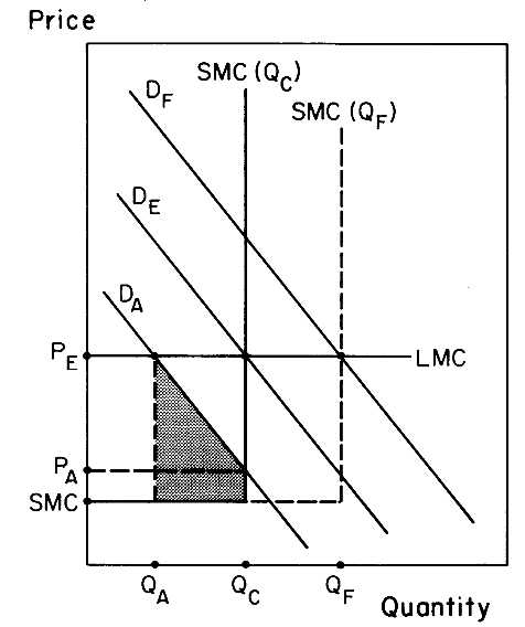
2.1. The future price is likely to be PK [where DF = SMC(QN .)]. DA = actual current demand, DE .: = erroneous earlier forecast of current demand, DF ,. = forecast of future demand, SMC(QC ) = short-run marginal costs with capacity QC , SMC(QF ) = short-run marginal costs with capacity QF , LMC = long-run marginal cost. The hatched area is the short-run loss of using PE ,: rather than PA as the current price.
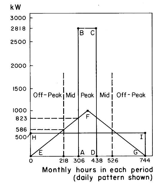
2.2. Patterns of kilowatt demand by time of day.
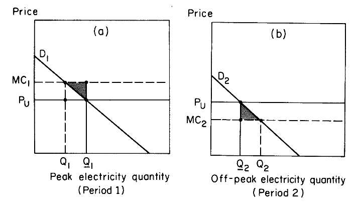
2.3. The efficiency gains from peak-load pricing (shaded):
(a) period 1 (peak), (b) period 2 (off-peak).
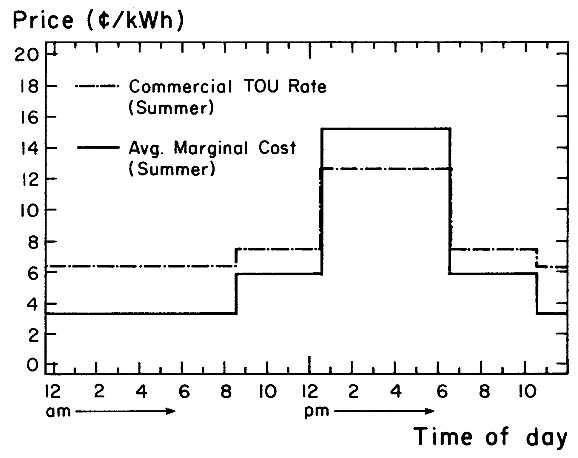
2.4. PG&E summer marginal cost and commercial TOU rates.
THREE
Issues in Public Utility Regulation
Richard J. Gilbert
I. INTRODUCTION
Although the roots of public utility regulation are buried in the political economy of the struggle for control of power, a main economic benefit of regulation has been, until recently, to provide a stable environment for investment in large-scale facilities. Regulation has the characteristic of an implicit contract between the regulated firm and its ratepayers (see Goldberg, 1976). The terms of this contract have provided insurance for the regulated firm against changes in factor costs and demands. The firm had the obligation to build new facilities to meet demand; in return for this responsibility, ratepayers implicitly agreed to guarantee the firm a reasonable rate of profit.
Until the mid-1960s investment in ever larger facilities made economic sense as each increment in scale brought lower costs of production. According to Kendrick and Grossman (1980), from the postwar period until the mid-1960s, public utilities (electric, gas, and water) showed the highest rate of total factor productivity growth of any two-digit Standard Industrial Classification code industry surveyed by the Department of Commerce. The average rate was 4.9%/year compared with 2.0%/year for all private domestic business and 2.5%/year for manufacturing overall.1
From 1966 to 1976 electric and gas utilities scored an average productivity loss of 0.2%/year, while productivity increased an average of 1.4% for all business. Also during this period and through the decade of the 1970s, a number of factors worked against what had been the uncon-
tested argument that larger plants were better plants. Inflation and environmental concerns weighed heavily against large-scale facilities. Some of the problems with the new plants were purely technical. The largest plants were not performing at expected capacity utilization rates. Other reasons were economic. Increases in construction costs and in the costs of financing pushed up sharply the capital costs of new technologies, while fuel costs soared.
The record of total factor productivity in the electric power industry has been determined largely by technological advances, demand growth, and resource prices and availability; however, regulatory incentives have also played an important role.
In practice, ratemaking has not generally followed the rate-of-return model. Rate-of-return regulation requires an evidential hearing. In the golden years of electric utilities, when costs were declining, requests for rate hearings were few. Rates of return earned by utilities sometimes exceeded the rates that would have been determined if the utilities were closely regulated, but prices were stable and the initiative for a rate hearing was often absent (Joskow, 1973). In those days many rate hearings were initiated by utilities to lower rates as a reflection of improved operating economics. Regulatory lag with declining costs worked in favor of the utilities and encouraged risk taking in new investments. Utilities had the option of requesting a rate hearing, so rate-of-return regulation provided a safety net for utility earnings, while regulatory lag made higher earnings a possibility. Utility managers had an incentive to invest in the most cost-effective technologies, because lower costs were reflected in higher earnings.
The situation changed drastically in the late 1960s as higher costs led utilities to request frequent and substantial price increases. Regulatory lag and the concerted opposition of ratepayers to further price increases acted in this period to lower earned rates of return (Joskow, 1974). The regulatory process discouraged new investment, and utilities concentrated their efforts on ensuring that revenues would be available to compensate past expenditures.
Although determination of allowed rates of return continued as a main issue in regulatory proceedings, a focus of recent policy has been on the regulation of the rate base. Major issues in the determination of the rate base are (1) allowance for funds used during construction (AFUDC) and (2) prudence. AFUDC is a holding fund for accumulated interest on expenditures for a plant that is not yet operational. The need for an AFUDC account is predicated on the policy that earnings should not be allowed for equipment that is not "used or useful." When a plant becomes operational, both the investment costs and the interest costs are included in the company's rate base. But until that event, AFUDC is a form of deferred gratification for the utility.
In the days when nominal interest rates were under 10% and the average time required to build a new plant was under five years, the opportunity cost of funds used for construction of new facilities was a small expense. But with double-digit interest rates and double-digit lead times for new construction, this item has become a major component of the costs of new plants. For example, of the $5.7 billion spent on units 1 and 2 of the Diablo Canyon nuclear power plant, approximately $2.0 billion, or about 35%, is in the AFUDC category (Chapter 7).
Increasingly, regulators have been questioning the propriety of expenditures and have been holding management to "prudence" accounting before costs can be entered into the rate base. The combination of regulatory lag, rate base accounting conventions and prudence requirements caused some utilities to be unable to earn rates of return sufficient to cover the cost of capital for new facilities (despite apparently adequate "allowed" rates of return), while many others faced the risk that future revenues would not fully compensate past and anticipated future expenditures.
The result was a regulatory incentive package that discouraged investment in baseload facilities and encouraged conservation programs to help avoid new investments. For much of the past decade such a policy made sense. The marginal cost of new investment exceeded the average price of electricity, which is. based on the average cost of existing production facilities. To the extent that consumers react to current average prices (see Chapter 2), they underinvested in conservation and therefore encouraging conservation made sense. A regulatory policy that discouraged new investment also made sense in an environment where demand growth was expected to slow and reserve margins were swelled by recent completions of large baseload plants, as occurred in recent years in California (Chapter 4).
However, the incentives created by the restrictive regulatory policies of the recent past will not serve the needs of the next decade. As John Quigley argues in Chapter 8, some operative conservation programs are questionable on economic grounds with the present cost structure of the industry. A long-term solution to electric power needs will require additional investment in baseload facilities. How can regulators convince utility managers that it is in the interest of their stockholders to absorb the risks of investing in new baseload plants?
The regulatory disincentives of the recent past have been most severe for large investment projects with long lead times. Although the most obvious problems, such as the failure to compound interest allowances for funds used for construction, have largely been alleviated, many disincentives remain that make large-scale investments unattractive for regulated utilities. The regulatory contract in effect during the past two decades could be summarized as "break even if it works, lose money if it
does not." The prudence doctrine, as it has been applied in many regulatory controversies, is an example of this implicit contract. Needless to say, the expected return from uncertain, long lead time projects under this implicit regulatory contract is not very enticing.
The regulatory challenge in the public utility sector is to provide an environment that allows firms to correctly weigh the risks of alternative new plants and to select the most cost-effective technology, whether that be nuclear power, coal, wind, solar, cogeneration, or conservation. There are two components to this challenge. One is to provide producers with an incentive structure that encourages efficient risk taking. The other is to encourage an industrial structure in the electric power industry that is most conducive to the attainment of technological efficiency.
II. CONCENTRATION OF POWER AND THE BENEFITS OF MERGERS
The market structure of the electric power industry is little changed from the structure that existed in 1935, when Congress passed the Public Utility Holding Act. Concerned by mergers and the creation of holding companies in the stock market of the 1920s, Congress effectively impeded capital restructuring in the electric power industry with the passage of this act. Although mergers have played a major role in shaping the nation's industrial structure and that of utilities in telecommunications that were not directly targeted by the Public Utility Act, the electric power industry has been (until quite recently) almost untouched by merger in the postwar period.
A common justification for the regulation of public utilities is their status as natural monopolies, and potential abuse of monopoly power is one argument in favor of an antimerger policy for electric utilities. The natural monopoly argument is not generally accepted, but even if it were valid, a closer examination shows that it does not justify a merger prohibition.
Monopoly power in electricity is local, arising primarily from economies of density in distribution networks. Horizontal merger neither increases nor decreases the extent of this source of monopoly power, which in any case is regulated by local public utility commissions. Although merger waves have triggered concern about excessive economic (and political) concentration in our economy, the isolation of the electric power industry from merger activity has not been without cost for this industry and consumers. Utilities have market power in their local distribution networks, but in electric power generation they are a relatively unconcentrated group. In 1980 the four largest electric power companies accounted for about 17% of the electric power sales of all class A
and B investor-owned public utilities.2 At about the same period of time, some typical four-firm concentration ratios for capital intensive industries are 28% for petroleum refining, 42% for blast furnaces and steel mills, 85% for flat glass, 31% for cement, 84% for turbines and turbine generator sets, and 92% for motor vehicles. S Of a total of 114 industries defined by the Census of Manufacturing under the headings of "Petroleum and Coal Products," "Primary Metals," "Machinery except Electrical" and "Electric and Electronic Equipment," only 14 had four-firm concentration ratios in 1982 that were equal power utilities. These industries typically involved specialized products (e.g., "industrial patterns") or products that covered a wide range of applications (e.g., "blowers and fans").
Concentration ratios are only a weak indication of the role of firm size in markets. These ratios do not account for the magnitude of transportation costs that might inhibit competition by geographically separated firms, and they are sensitive to arbitrary classifications of industry products. Nonetheless, an inspection of typical concentration ratios leads to the conclusion that the electric power industry is exceptional in the extent of its industry fragmentation, and this is particularly striking given the importance of scale economies in this industry. This observation has been made by others, including Primeaux (1975), Weiss (1975) and Joskow and Schmalensee (1984), and it is central to proposals advocating restructuring and deregulation of electric power generation.
An indicator of efficient firm size is the relation of firm assets to the size of their new investments. A rule of thumb is that the capacity of a minimum efficient-scale unit operating plant should be no more than about 20% of a firm's installed capacity before the unit is built. In the electric power industry a unit refers to a turbine-generator combination. It differs from a plant, which may contain more than one unit. If the unit size exceeds 20% of a firm's installed capacity, planned and forced outages will impose problems of reliability for the firm's supply system, and unless demand growth is very high or the unit displaces existing capacity, capacity utilization may be unacceptably low.
Table 3.1 shows the relation of utility size to the size of "pioneering" generating units over the past three decades. The table shows the percentage of firms for which the pioneering unit size is less than the indicated fraction of the total generating capacity of the firm.
Until recently, larger unit sizes resulted in lower average costs of producing power, and therefore the largest planned units were indicative of the frontier of generation technology. In Table 3.1, the pioneering unit
size is calculated as the average of the largest 25% of all units that began operation in the four, five and six years following the indicated date. This figure is representative of the largest plants in the planning and construction phase for each date. For example, the average of the largest 25% of units commencing operation in 1979, 1980, and 1981 is 769.5 MW, which is the pioneering unit size indicated for 1975 in Table 3.1.
The universe of electric power generating firms in Table 3.1 is taken to be the total for each year of all class A and B utilities that produced their own power. Table 3.1 shows that only a very small subset of all class A and B utilities could pass the 20% test for a new capacity addition. In 1955 the pioneering unit size was about 325 MW. In that year, only three firms had a total generating capacity in excess-of 3,250 MW, which would make the pioneering unit size equal to 10% or less of the size of the firm. Nine firms had a capacity in excess of 1,675 MW and therefore could pass the 20% test. This was less than 4% of all class A and B electric power utilities.
The 20% test was met by only a small percentage of the electric utility industry over the period 1955 to 1980. Growth in utility systems and a decline in the sizes of new units being built increased the fraction of the industry that could meet the 20% test to about 18% by 1980, but this is still only a small fraction. Only about 62% of the electric power firms in the industry in 1980 had a total generating capacity less than the size of a pioneering unit.
Actual experience in private industry with the relationship between firm size and the magnitude of investment projects provides a test of the "20% rule" and offers a benchmark for the evaluation of efficient electric power utility size. This comparison is necessarily imperfect. Circumstances differ greatly from one industry to another. A function of utility regulation is to provide financial stability for new investment, and thus utilities might be expected to be more inclined to undertake large projects. Nonetheless, experience in unregulated markets should provide an indication of how market forces influence firm size and this should be at least a guide for efficient market structure in the electric power industry.
Table 3.2 is a summary of the results of a survey of investment projects in different industries. In the petroleum industry, the largest project identified in the survey was a grass-roots, integrated petrochemical complex.4
Consistent with the prevailing refinery situation, no such projects were listed as currently under construction. However, if one were built, its estimated cost for 250,000 barrels/day capacity would be in the range
of $1.5 to $2.0 billion (1983 dollars). Upgrading an existing refinery is both more likely and considerably less expensive (Bowen, 1983). This is a very large undertaking, but even the high end of the cost estimate represents less than 10% of the total assets of the largest oil companies. Investment projects surveyed that were actually under way typically represented no more than a few percent of the assets of the firm responsible for the project (Cantrell, 1983; The Petroleum Encyclopedia, 1983).
Trade reports on the aluminum extraction and refining industry indicated investment projects as large as $2.5 billion (1983 dollars), but the largest project actually undergoing construction was $1.5 billion (the $2.5 billion project was deferred at the time of the survey). The $1.5 billion project was a refinery/smelter constructed as a joint venture with Alcoa and Shell Brazil, a subsidiary of Royal Dutch Shell (Engineering and Mining Journal, 1983). The combined assets of the two companies were about $37 billion in 1983, so that the project represented about 4% of the partners' total assets.
The largest projects in the manufacture of iron and steel products are grass roots fully integrated steel complexes. Only about a dozen of these complexes have been built worldwide since 1950, and only two in the United States. The cost could be as high as $3 billion, which would be about 30% of the assets of U.S. Steel. More common are investments in facilities such as oxygen furnaces and coke ovens, which cost up to about $200 million, or no more than 10% of the assets of a moderate-sized steelmaker (Miller, 1977).
In the automobile industry, the launching of an all new platform for a new vehicle can cost upwards of $1 billion. Chrysler estimated that a new line of front wheel drive vehicles would cost the company $1.2 billion (Lambert, 1979) in 1981 dollars and budgeted a similar amount in 1983 for the development of its minivan (Lapham, 1982).
The cost of a large baseload coal or nuclear plant investment can exceed the pre-investment assets of the larger electric power companies. This magnitude of risk exposure, as measured by the ratio of investment to firm size, is not typical in private industry. Although Table 3.2 shows some investments in the private sector that reach as high as 75% of firm assets, these pertain to unusual circumstances. In the case of iron and steel the figure is for a project that was neither planned nor attempted in the industry for many years. The 40% figure in the aluminum industry was for a project undertaken by a partnership of two firms whose total assets were about 25 times the project size.
The surveys summarized in Table 3.2 are only anecdotal and no doubt cases exist in which private firms have undertaken investment programs that are large both in absolute terms and as a fraction of the size of the firm. Nonetheless, the results summarized in the table
generally support the 20% rule of thumb. They also illustrate the extent to which risk-taking in the electric power industry, as measured by the relation of project to firm size, is unusual relative to the unregulated sector of the economy. Although surveys indicated that in the unregulated sector the largest projects were generally undertaken by the largest firms, there were many instances in the electric power industry in which large baseload generating plants were constructed by relatively small firms. Thus Table 3.2, which concentrates on the larger firms in the industries surveyed, probably understates the extent of risk exposure in the electric power industry.
One way that electric power utilities have escaped the 20% rule-of-thumb limitation is to form joint ventures for investment in new facilities. A nuclear plant may have several partners. Although joint ventures are not uncommon in private industry and provide institutional vehicles for sharing the risks associated with a major new investment program, they also introduce a host of other problems that stem from the coexistence of partners, each with different objectives, management approaches, and legal constraints.
A case in point is the Fitchburg Gas & Electric Company. Fitchburg Gas & Electric is a part owner (0.9% of unit 1) of the Seabrook nuclear power plant. Headquartered in Canton, Maine, the company has about 200 employees, total assets of $86 million, and revenues of about $50 million/year. Seabrook is well known as one of the most problem-plagued nuclear facilities in the nation. Begun with a cost estimate of several hundred million dollars, more than $5 billion has been spent on unit I alone, and though now completed, it is uncertain whether it will ever be operated.
Seabrook is a joint venture among several utility companies, including Fitchburg Gas & Electric. Although Fitchburg owns less than 1% of the Seabrook plant, its share amounts to a liability of about $50 million, or more than one-half of its assets. Clearly, partnering did not succeed in reducing the risks to Fitchburg Gas & Electric to an acceptable level. Moreover, the spreading of risks that is the objective of joint venture also prevents one of its greatest hazards. With many partners, the temptation is great to abandon a project that appears to be in trouble, leaving the burden of coast overruns to the remaining partners. This limited loyalty can add to the problems of financing and managing a large joint venture.
III. REGULATORY INCENTIVES AND DISINCENTIVES FOR INVESTMENT
The participation of utilities in investment projects that are much larger than would be considered reasonable by the 20% rule and the existence
of complex joint ventures are consequences of the regulatory conventions that have dominated the evolution of this industry. Regulatory practice in the past has provided protection to utilities by ensuring that revenues would be adequate to cover costs. This allowed utilities to take risks and exploit economies of new investments, even if these risks were very large relative to the standards of private industry. This implicit regulatory contract worked effectively in times of stable technology and declining costs, when mistakes rarely produced instances of rate shock for customers, and when predictable reserve margins made capacity planning a comparatively simple task.
Rate-of-return regulation is a version of cost-plus contracting. The standard regulatory formula generates a return to the utility that is directly proportional to the utility's incurred costs. Operating costs are compensated on an essentially one-for-one basis. Capital costs are compensated by permitting annual charges equal to the allowed rate-of-return on total assets. There are many differences in regulatory procedures and many complications in the ratemaking process (see Chapters 2, 4, and 5) but the essential fact is that rate-of-return regulation is a cost-based approach to ratemaking.
Allowing revenues in proportion to costs is hardly conducive to efficient operations, and with skyrocketing costs for new construction programs it is not surprising that regulators have begun to scrutinize the record of utility performance. Prudence is an old concept in regulatory law that provides for inclusion in the rate base only those expenditures that represent acceptable managerial judgment, but with the large cost overruns encountered in recent years the prudence doctrine has taken on new life.
The appeal of the prudence doctrine is that management should be held responsible to exercise good judgment, and ratepayers should not be penalized for imprudent behavior. Of course, the determination of behavior that is imprudent is not easy. Also, the recent vigorous application of the prudence doctrine can be criticized as a change in the rules of the game. If prudence was not an issue at the time that the expenditures were made, application of the prudence doctrine cannot be justified by its incentive effects on those expenditures. The efficiency consequences can apply only to future expenditures.
The determination of imprudent behavior is always difficult, but the stimulus to search out imprudence increases with the size of the rate shock following the completion of a new plant. Mistakes are not a new phenomenon, but they were easier to forgive in times when prices were stable. Until recently, completed plants typically were entered into the rate base at full cost without an audit of management performance. Despite the obvious merits of pruning out imprudent behavior, the current vigor with which management is held responsible for prudent
performance represents a change in the structure of the implicit regulatory contract.
Some form of prudence accountability should be present in any efficient regulatory framework. A free market has its own prudence doctrine, because the costs of imprudent investments are borne directly by the investor. The current trend in the application of the prudence doctrine has two serious flaws. The first is that while negligence is punished, there is no provision for rewarding outstanding management performance. The prudence cry has been a reaction to price movements; it has not been applied as a true gauge of management performance, and its methods include a stick, but no carrot.
The second major flaw in the application of the prudence doctrine is that it punishes stockholders directly and management only indirectly. A typical application of the prudence concept is to disallow certain costs from inclusion in the rate base. This means that the firm cannot earn revenues on these costs and the market value of the firm is correspondingly reduced. The direct burden of this action falls on the shareholders of the company.5 Managers suffer to the extent that their well-being is correlated with the market value of the firm. However, the ownership of shares by utility managers is very small, and managerial salaries in the utility industry are not usually directly affected by application of prudence. Thus the shareholders feel the pain of prudence in their pocketbooks, while managers take it on the ego.
To the extent that management can be held accountable for company performance, management should share in the fruits of their activities. This means paying for clear mistakes and receiving tangible rewards for superior performance. A managerial incentive package would not be costly to ratepayers because managerial salaries are a small fraction of total expenses. But the incentive effects of such a strategy could bring sizable rewards over the longer term to both ratepayers and shareholders.
Regulatory reform in the public utility sector is essential not only to improve the incentives for efficient operations, but also to exploit the potential gains from restructuring in this industry. Merger activity can reduce the size of new investments as a fraction of firm size and in this way mergers can improve the statistics of risk exposure in public utilities. But an improvement in this statistic is unlikely to bring real gain to ratepayers and shareholders unless it is combined with measures that reward efficient behavior. For example, current regulatory practice compensates utilities in proportion to the size of the "used and useful" rate base. It does not reward utilities for minimizing cost or for seeking out
the most cost-effective supplies, unless rate regulation is adapted to respond to such behavior. Under traditional regulatory practices (and depending on allowed rates of return and the extent of capacity utilization), utilities could have an incentive to merge for the purpose of expanding the size of the rate base. If regulation does not adapt to encourage efficient behavior, and particularly if no new investments are planned for several years, there is little reason to expect productivity gains from such a merger. But if restructuring of the industry is combined with regulatory reforms that provide incentives for efficient management, there is cause to expect that structural change will be motivated by desires to improve operating efficiencies and that these changes will eventually impact positively on ratepayers and shareholders.
IV. A PROPOSAL FOR REFORM
The Public Utility Regulatory Policies Act of 1978 (PURPA) was a watershed event for the regulation of electric power. PURPA allows independent, unregulated producers to enter the electric power business, and the consequences can be dramatic. Drawing a parallel to telecommunications, the deregulation movement in that industry began when the Federal Communications Commission approved the entry of an independent carrier into the regulated private-line business. It was then only a matter of time until entry into regulated general long-distance services was allowed. What had started as a ripple in the industry turned into a major current of change with the entry and expansion of new independent carriers.
PURPA limits entry to cogenerators and to small power production facilities using certain "soft" technologies with a capacity of less than 80 megawatts (MW).6 Also, qualifying facilities can sell power only for resale.7 Despite these limitations, independent power producers in some states have responded vigorously to the prospects of selling electric
power. The figures shown in Tables 3.3 and 3.4 aggregate the cogeneration and small power production for the service areas of PG&E, SCE, and SDG&E. They indicate a staggering potential contribution to the electric power production capacity of California. The California Energy Commission estimates that the dependable electricity production capacity of the state, excluding small power producers, self-generation, and imports, is approximately 46,000 MW, of which about 38,000 MW are in the PG&E, SCE and SDG&E service areas (California Energy Commission, 1989). The total on-line and potential cogeneration and small power production capacity indicated in Table 3.3 is almost 50% of the dependable capacity in PG&E, SCE, and SDG&E service areas. It is almost ten times the capacity of the Diablo Canyon nuclear power plant (2,190 MW for both units).
Much of the capacity indicated in Table 3.3 is potential, not actual. Of the total of 18,000 MW of actual and planned capacity, 1,664 MW were on line at the end of 1984. Although only a small fraction of the total, this is still a significant contribution to the electric power capacity of the state. Furthermore, Table 3.4 shows rapid growth in the amount of online cogeneration and small power production. Actual capacity more than doubled in the two years from the end of 1984 until the end of 1986. By the third quarter of 1989, the amount of on-line power doubled again. By the third quarter of 1989, outstanding project commitments (which are the total of projects on line, in progress, and projects with signed letters of agreements), represent yet another doubling of actual capacity.
The response of cogenerators and small power producers to the window of opportunity created by the Public Utility Regulatory Policies Act of 1978 was nothing short of phenomenal. Of course a major factor in the growth of independent power production in California was the result of the attractive terms of Standard Offer No. 4, which guaranteed long-term purchase prices that are much higher than the near-term marginal cost of electricity. Standard Offer No. 4 has since been suspended by the CPUC, but many of the projects summarized in Tables 3.3 and 3.4 have the benefit of Standard Offer No. 4 or similar contracts that offer high long-term purchase prices.
The phenomenal rate of growth of cogeneration and small power producers in California is unlikely to be sustained when long-term purchased contracts such as Standard Offer No. 4 are replaced with contracts that offer less favorable terms. The incentives for independent power production will be less attractive, and the pool of favorable sites for independent power has been diminished by the growth that has occurred. Nonetheless, the experience with independent power in Califor-
nia summarized in Tables 3.3 and 3.4 is a clear indication that independent power production can make a large contribution to electric power needs, at least in the state of California. The advent of PURPA has been a major reform of utility regulation, which, despite its limitations, has the potential for significant change in the structure of the electric power business.
Deregulation is an economist's motherhood and apple pie, but PURPA, as it is currently implemented, introduces as many problems as it solves. The size and technology restrictions aggravate the current regulatory bias against large-scale facilities. The challenge of regulation is to provide a climate that encourages investment in the most cost-effective alternatives. The current regulatory environment does not do that and PURPA does not help.
Another PURPA problem is the restriction of power only for resale. Qualifying facilities (QFs in the PURPA vernacular) do not compete in the general market for electric power. They compete only with a utility's "avoided cost"—an elusive concept that is transformed into reality after an arcane calculation by a regulatory commission. Furthermore, regulatory restrictions limit the involvement of utilities in qualifying technologies, so that competition in the PURPA territory is even more limited.
The current approach toward contracting for qualifying facilities imposes regulatory risks on both the QFs and the utilities. The QFs have to forecast avoided costs, unless they can enter into long-term contracts at set prices. With long-term contracts at fixed prices, utilities and rate-payers have to assume the risk that the future value of the PURPA energy will be different from its contractual cost and that the resulting amount of power produced will be more or less than is desired.
With only short-run or spot prices for avoided costs, QFs have to face the risk that future prices may not be sufficient to cover capital costs, and this uncertainty may make capital more difficult to obtain. QF proponents can argue that regulation is asymmetric in this situation, because regulation at least nominally reimburses costs incurred by public utilities and provides some protection from risk, while short-run pricing for QFs does not provide equivalent insurance.
The PURPA regulatory process imposes different risks on utilities. Utilities do not have the option of taking a risky contract that would allow them to earn above-normal profits (as well as losses) from new investments. Also, regulatory risks fall on the utility whenever it guarantees a rate structure to a QF, whether the rate structure is long-term or spot. The utility must recover these revenues in a regulatory process that experience has shown is not without risk. Having agreed to contracts with QFs, the utility is a residual claimant to earnings that are left
over after the QFs are paid. The natural response for utilities to this situation is to pursue a yet more cautious investment policy—one that minimizes the amount of capital at risk.
Thus the effect of PURPA may be to further increase the bias against large investment projects. Also, with utilities barred from cogeneration projects and with no incentive to build large plants, we may find regulated utilities more in the position of being energy brokers for independent power producers, with their own investments reduced to quite limited programs.
Despite its limitations, PURPA brings a major regulatory innovation to the electric power industry with significant opportunities for positive reform. The avoided cost pricing methodology advanced in PURPA is a powerful alternative to the existing rate-of-return approach to public utility regulation. Rate-of-return regulation is essentially unworkable. When it is applied to the letter, it creates sharp differences between the technology choices favored by stockholders and the choices that either minimize customer revenues or maximize productive efficiency. Simply stated, whenever the allowed rate-of-return exceeds the cost of capital, stockholders should favor the most capital-intensive technology because this maximizes the profits of the firm. When the allowed rate-of-return is less than the cost of capital, stockholders favor the least capital-intensive technology if growth must occur, and they would prefer not to invest at all if that were an acceptable outcome (see Chao, Gilbert, and Peck, 1984).
Rate-of-return regulation provides little in the way of incentives to hold down costs. Also, rate base regulation is more risky for projects with long lead times and large capital expenditures, and hence rate-of-return regulation discourages investment in these types of technologies. If utility managers could be convinced that future regulatory policy would allow generous earnings relative to the cost of capital and that future expenditures would be guaranteed to be included in the rate base with no penalties, the bias against large projects would turn completely around to a stimulus for investment in such projects. But it is difficult to see how regulatory commissions can convince utility managers that the problems of regulatory risk with respect to large, long lead time projects will be solved and that the regulatory insurance policy so reliable years ago will be reinstated. Without such a commitment, it is likely that rate-of-return regulation will continue to include a bias against large investment programs for some time to come.
An extension of the avoided-cost methodology introduced by PURPA allows a mechanism for reform of public utility regulation in a way that would not discriminate against projects of different sizes. This proposal is a modification of the recommendation given by David Roe (1985), who
suggests that (short-run) avoided-cost pricing replace rate base regulation for regulated utilities, as well as being available to independent power producers under PURPA. The advantage of this proposal is that short-run avoided cost, if computed properly, is a measure of system marginal cost, which is the true value of another unit of power on the electric power system.8 A criticism of short-run avoided-cost pricing is that the variability and unpredictability of future rates frustrates generation planning and makes it difficult to raise capital for new projects. The following proposal is an attempt to deal with this problem, while preserving the efficiency advantages of Roe's proposal.
Short-run avoided-cost pricing is desirable because of the difficulty, mentioned above, that a fixed-price offer may bring either too much or too little generation relative to the needs of consumers. A fixed price that is too high will result in too large reserve margins, and with excess capacity the system marginal cost is likely to be below the fixed price. The converse may occur if fixed prices are too low.
However, efficient production requires only the equality of prices and marginal costs for those generation decisions that are on the margin. Fixed prices are not inconsistent with the attainment of economic efficiency if it is possible to produce more or less power and receive a price equal to the short-run system marginal cost.
To see how this may be accomplished, suppose a firm (public utility or otherwise) is considering a project which will add a production capacity of K megawatts with a cost structure
|
C (q , K) = b K + vq |
for q < K |
where q is actual output in megawatts, b is the capital cost per unit of capacity, and v is the variable cost per unit of actual output.If short-run pricing prevails, future prices will depend on demand and supply conditions and will be uncertain at the time the new plant is under consideration. The plant should operate only if the price exceeds its variable cost, v. If the future price at time t is P(t), the plant will earn net revenues of P(t)- v for every megawatt it produces when P(t) exceeds v, and it will stand idle whenever P(t) is less than v. The plant will be built only if expected net present value revenues, adjusted for risk, exceed the capital costs (including all financing costs). Price risk can be removed by offering a guaranteed price P g (t). The firm then will produce whenever P g (t)> v;however, this is inefficient if the system marginal cost is less than v .
This difficulty can be corrected with the following scheme. The regulatory commission allows the firm to sell a fraction, a, of its production
capacity at the guaranteed price P g (t). The remaining capacity, (1-a )K, is available for purchase at the spot price P(t ), which is set equal to the short-run system marginal cost. The firm should sell this power only if P(t)> v: hence the firm operates efficiently with respect to production in excess of the contracted amount a K.
In addition, the firm is offered the following bargain. If for any reason the purchaser does not want to buy all of the contracted power aK (assuming that it is available), then the firm will be offered a price P o (t) as a payment for not producing. The firm need not accept the offer. However, if P o (t) is set equal to the difference between the guarantee price P g (t) and the system short-run marginal cost P(t ), a profit-maximizing firm would accept the offer only if it were economically efficient to do so from the standpoint of total system costs. To see this, note that if the firm chooses to produce, it receives the guaranteed price P g (t) and earns P g (t) -v /megawatt. If it accepts the bargain and stands idle, it receives P g (t) -P(t) for each megawatt that it does not produce when q(t) is less than aK. Accepting the bargain is a good deal for the firm if P g (t) - P(t)> P g (t) v, or if v P(t ), but this is exactly the condition under which the firm should not produce, because the firm's short-run marginal cost exceeds the system's short-run marginal cost.9
This proposal of a combined guaranteed price for a contracted amount of production, along with a spot price for either increases or decreases in production, has several advantages.
• The offer assures the investor guaranteed revenues equal to Pg (t)a K if the plant is capable of producing at least K. The guaranteed payment is an insurance policy for the firm.
• The opportunity to sell more at the spot price P(t) or to sell less in exchange for the payment Pg - P(t) permits the firm to increase its net revenues above the level implied by the guaranteed price. The firm will trade more or less than the contractual amount only if it is profitable to do so. The contractual revenues are only a floor on the firm's total earnings.
• The purchaser can guarantee payments of no more than Pg (t)aK by refusing to engage in spot trades. The purchaser will buy more only if the seller can generate the additional power efficiently.
• The purchaser can reduce its payment obligations by exercising the right to buy less than a K at a price of Pg (t)- P(t)/megawatt, provided the seller accepts the offer. If the seller agrees not to produce
at all, the purchaser's maximum payment is not Pg (t) a K, hut rather [P g (t) - P (t)] a K
• This proposal retains regulatory jurisdiction in those areas where regulation may serve a useful purpose These are:
Long-Run Capacity Planning
A criticism of deregulation proposals in the electric power industry is that an unregulated market may be less efficient than an administered market in planning capacity additions to meet demands. This argument would have little basis if futures markets existed for electric power, but they do not and their appearance is not likely (a deregulated market is more likely to develop long-term contracts for electric Power supply, with elements similar to those suggested in this proposal). Furthermore, for large capacity additions, the market criteria for profitability do not coincide with the social calculus for an efficient investment. The market compares total present-value revenues against total present-value costs. The social calculation relies on total present-value benefits, which exceed the revenues earned for a large increment to capacity.
For these reasons it may be desirable for a regulatory body to retain some control over the amount of planned capacity additions. The price guarantee provides a means by which this may be accomplished. By increasing or decreasing the guarantee price and the share a regulator can control the amount of capacity additions by altering the profitability of new investment.
Standard Offer No. 4 has been held as an example of the problems of offering a guaranteed price. Reserve margins in the next decade are expected to be adequate and the amount of independent power responding to the price offer will be a surplus on the electric power market. If this is true, it merely argues that the guaranteed price is too high. In practice the guarantee price should be flexible, adjusting to match perceived capacity needs with indicated supplies.
Electric Power Tariff Structure
The proposed pricing schemes affect only the supply side of the electric Power market. Regulators are free to choose customer prices at will, subject to the constraint that revenues are sufficient to cover costs (if the regulatory commission cannot run a deficit). Another constraint on the regulatory commission is that the price structure should not encourage end users to abandon the public supply system and produce for their own needs. This bypass problem is an indication that some consumers are subsidizing others (because they are paying more than their "stand-alone" cost of supply), and it is already emerging as an important issue in electric power regulation (see Chapter 4).
Cross-subsidization is endemic to regulated industries; indeed, some would say it is basic to the regulatory process. Posner (1971) describes regulation as an institution that allows a system of taxation and subsidies. Much of the cross-subsidization present in regulated electric power tariffs would be eliminated if the electric power industry were opened to competition. A free market would bring supplies to those customers who are paying more than their incremental cost of production, at the expense of those who are paying less.
Cross-subsidies exist sometimes for political reasons, but other times for reasons of perceived fairness. Complete abandonment of the power to cross-subsidize would eliminate the flexibility to respond to these concerns. The proposed pricing system preserves some regulatory flexibility for end-user pricing, although constrained by market realities.
PURPA may revitalize the electric power industry, bringing new technology and new vigor to the market. It also may bring a return to the early years of this century, when a proliferation of backyard power plants of inefficient scale with quickly obsolete technology interrupted the development of a new industry. The pricing proposal described here provides an opportunity to extend the structural changes inherent in PURPA to the industry at large. The proposal would avoid a regulatory system that discriminates against particular generation technologies and replaces it with a system that allows competition among all potential suppliers of electric power, while retaining important aspects of regulatory oversight for the planning of electric power supply and for fairness (consistent with costs) in the pricing of electric power.
REFERENCES
Bowen, C. (1983). "Petrochemical Units Benefit from Integration, Flexibility." Oil and Gas Journal, Vol. 81, No. 15, April 11, pp. 100-104.
Cantrell, A. (1083). "Worldwide Construction." Oil and Gas Journal , Vol. 81, No. 17, April 25, pp. 105-142.
California Energy Commission (1989). 1988 California Electricity Report . June, P106-88-001. Sacramento.
Chao, H. P., R. J. Gilbert, and S. C. Peck (1984). "Customer and Investor Evaluations of Power Technologies: Conflicts and Common Grounds." Public Utilities Fortnightly , Vol. 113, No. 9. April 26, pp. 36-41.
Dun & Bradstreet (1982). Dun’s Business Rankings ; 1982. Dun & Bradstreet Corporation, Parsippany, N.J.
Engineering and Mining Journal (1983). "Mining Investment 1983," Vol. 184,No. 1, January, pp. 43-63.
Goldberg, Victor P. (1976). "Regulation and Administered Contracts." Bell Journal of Economics , Vol. 7, No. 2, pp. 426-448.
Joskow, Paul (1973). "Pricing Decisions of Regulated Firms: A Behavioral Approach." Bell Journal of Economics , Vol. 4, No. 1, pp. 118-140.
Joskow, Paul (1974). "Inflation and Environmental Concern." Journal of Law and Economics , Vol. 17, No. 2, pp. 291-327.
Joskow, Paul, and Richard Schmalensee (1984). Perspectives on Power .
Kendrick, John W., and Elliot S. Grossman (1980). Productivity Trends in the United States: Trends and Cycles . Baltimore: Johns Hopkins Press.
Lambert, P. (1979). "Chrysler Considering FWD for all New Models." Automotive News , August 27, No. 4771, p. 1.
Lapham, E. (1982). "Iacocca Sees a Delayed Recovery." Automotive News , November 26, No. 4943, p. 1.
Miller, J. (1977). "Ogishima: A New Steelworks for an Old One." I &SM, Vol. 4, No. 6, June, pp. 23-27.
Moody's Investors Service (1983a). Moody's Industrial Manual . New York: Dun & Bradstreet Corporation.
Moody's Investors Service (1983b). Moody's Public Utility Manual . New York: Dun & Bradstreet Corporation.
Pacific Gas and Electric Company (1989). "Cogeneration and Small Power Production Quarterly Report to the California Public Utilities Commission." Third Quarter.
The Petroleum Encyclopedia (1983).
Posner, Richard (1971). "Taxation by Regulation." The Bell Journal of Economics , Vol. 2, No. 1, pp. 22-50.
Primeaux, Walter J., Jr. (1975). "A Reexamination of the Monopoly Market Structure for Electric Utilities." In A. Phillips (ed.), Promoting Competition in Regulated Markets . Washington, D.C.: Brookings Institution, pp. 175-200.
Public Utility Regulatory Policies Act (1978). Public Law 95-617, 95th Congress, 16 USC 2601, 92 STAT. 3117-3173. Nov. 9, 1978.
Roe, David B. (1985). "QF Pricing: Issues and Implications." Presented at the Fifth Annual California Public Utilities Commission Conference, San Francisco, March 25.
San Diego Gas and Electric Company (1989). "Customer Generation Quarterly Report." Third Quarter.
Southern California Edison Company (1989). "Cogeneration/Small Power Production Quarterly Report to the California Public Utilities Commission." Third Quarter, September 30.
U.S. Department of Energy (1980). Statistics of Privately-Owned Electric Utilities in the United States .
U.S. Department of Energy (1986). Inventory Power Plants in the United States , DOE/EIA-0095.
Weiss, Leonard (1975). "Antitrust in the Electric Power Industry." In A. Phillips (ed.), Promoting Competition in Regulated Markets . Washington, D.C.: Brookings Institution, pp. 135-173.
|
TABLE 3.1 |
|||
|
Pioneering |
Number |
Percentage of Firms ith Ratio of Pioneering |
|
|
Year |
Size (MW) |
Firms |
0. 1 |
0.2 |
0.5 |
0. 75 |
1.0 |
All |
|
1955 |
324.8 |
237 |
1.3 |
3.8 |
17.3 |
27.0 |
34.6 |
100.0 |
|
1960 |
436.5 |
215 |
1.4 |
5.6 |
20.9 |
32.6 |
39.1 |
100.0 |
|
1965 |
792.4 |
192 |
0.0 |
3.6 |
17.2 |
30.7 |
38.0 |
100.0 |
|
1970 |
954.8 |
188 |
0.5 |
5.9 |
24.5 |
34.6 |
43.6 |
100.0 |
|
1975 |
769.5 |
185 |
5.4 |
15.1 |
40.5 |
54.1 |
60.5 |
100.0 |
|
1980 |
881.6 |
180 |
6.7 |
18.3 |
43.3 |
52.8 |
62.8 |
100.0 |
|
a SOURCES: U.S. Department of Energy (1980) and U.S. Department of Energy (1986). |
||||||||
|
TABLE 3.2 |
||||
Industry |
Projectb |
Project Sizeb |
Firm Assetsc |
Ratio of |
|
Petroleum |
Integrated |
1.5-2.0 |
27 |
0.06-0.07 |
|
Aluminum |
Smelter/ |
1.5 |
3.6 |
0.4d |
|
Iron and |
Integrated |
0.2-3.0 |
4.0 |
0.05-0.75e |
|
Motor |
New Model |
1.2 |
6.3 |
0.2 |
|
Electricity |
Large Coal |
3-6 |
3.6f |
0.85-1.7 |
|
a SOURCE: Moody's Investors Service (1983a and 1983b), Dun & Bradstreet (1982), and trade journals referenced in the text. NOTES:b Project and project size are the largest investments by major firms in the industry. c Asset size is the size of the third largest firm in the industry in 1982. d Project undertaken by a joint venture with combined assets of $37 billion. The ratio of project size to the partners' total assets was about 4%. e None of the largest projects were under construction or planned. f Asset size for electric power utilities only. g Asset size for all electric and combined electric and gas utilities. |
||||
|
TABLE 3.3 |
||||
Project Type |
On Line |
Signed |
Signed Letter |
Under Active |
|
Cogeneration |
788 |
3,827 |
89 |
4,196 |
|
Biomass/Solid Waste |
78 |
1,222 |
113 |
440 |
|
Solar |
26 |
140 |
17 |
27 |
|
Small Hydro |
181 |
661 |
6 |
327 |
|
Wind |
496 |
2,812 |
4 |
1,614 |
|
Geothermal |
95 |
504 |
— |
87 |
|
Total |
1,664 |
9,165 |
229 |
6,691 |
|
Grand Total |
17,749 |
|||
|
a SOURCE: California Public Utilities Commission. |
||||
|
TABLE 3.4 |
|
|
MW of Capacity as of |
|
Project Type |
Dec. 1984 On Line |
Dec. 1986 On Line |
Sept. 1989 On Line |
Sept. 1989 Commitments |
|
Cogeneration |
788 |
1,675 |
4,614 |
7,409 |
|
Biomass/Solid Waste |
78 |
274 |
629 |
1,480 |
|
Solar |
26 |
117 |
216 |
605 |
|
Small Hydro |
181 |
281 |
303 |
695 |
|
Wind |
496 |
1,234 |
1,357 |
3,599 |
|
Geothermal |
95 |
188 |
647 |
909 |
|
Total |
1,664 |
3,769 |
7,766 |
14,697 |
|
* SOURCE: Pacific Gas and Electric Company (1989), San Diego Gas and Electric Company (1989). Southern California Edison Company (1989). |
||||
FOUR
The Value of Rate Reform in a Competitive Electric Power Market
Richard J. Gilbert and John E. Henly
I. INTRODUCTION
The 1980s signaled a new pattern of competition in the electric power industry. Increased capital costs resulting from newly completed construction projects boosted utility rates at the same time that lower oil and gas prices and procompetitive legislation, led by the Public Utility Regulatory Policies Act, provided alternatives to utility-generated power.
These changes in utility costs and industry structure undermined the economic performance of California's electric rate structures (as well as those of other states). Features of California's rate structure that could be defended on economic efficiency grounds in the late 1970s and the early 1980s were impediments to economic efficiency in the late 1980s and, if not altered, will probably continue to have adverse consequences through the turn of the century.
The features of the current pricing system that are particularly troublesome in this new environment are: (1) the increasing block tariffs faced by residential customers, (2) the application of traditional cost recovery practices to recently completed construction projects, and (3) the subsidization1 of residential and agricultural customers by industrial and commercial customers. These features drive electricity prices away from marginal costs. As a result, businesses are driven away from least-cost
production techniques, and consumption decisions are distorted by prices that are removed from marginal costs.
Regulators and state legislators may, of course, pursue goals other than economic efficiency, but it is important from a policy standpoint to place a price on those goals. In this chapter we attempt to determine this price. We calculate that a failure to respond to recent changes in the utilities' cost structure in an economically efficient way would cost northern California's businesses and consumers approximately $400 million a year (levelized) over the 1987-2003 period. Extrapolating these results to the entire state indicates a cost of approximately 1 billion per year on a levelized basis.
Our results indicate the need for a coordinated approach to utility rate design. If utility revenues are required to cover costs, a change in the allocation of revenue responsibilities across customer classes alone cannot achieve significant efficiency gains without large distributional impacts. Moreover, changes in the pattern of cost recovery over time have limited scope for efficiency gains without large accompanying changes in customer rates. But it is possible to design an efficient rate structure that is distributed more acceptably if changes in customer rates are coupled with changes in the pattern of utility cost recovery over time.
In the next section we discuss qualitatively how changes in cost structure and technology have reduced the economic efficiency of electric rate structures similar to California's. Then we describe our methodology and the dynamic simulation model used to measure the effects of rate structure changes on economic efficiency. We measure the gain in economic efficiency that would result from changing the 1986 rate structure2 to marginal-cost pricing for a utility modeled after the Pacific Gas and Electric Company (PG&E), California's largest electric utility. We explore the efficiency effects of specific features of the California rate structure by "improving" them (in terms of economic efficiency) while holding other characteristics of the rate structure constant. We look at alternatives to traditional utility cost recovery practices, assuming uniform rate schedules. Revenue requirements are shifted among industrial, commercial, and residential rate classes using Ramsey and modified Ramsey criteria to determine how the allocation of revenue requirements among customer classes affects economic efficiency when marginal-cost pricing is not possible. Recognizing that political and equity constraints limit rate reform, we conclude the quantitative analysis by discussing a rate structure that achieves more than one-half of the efficiency benefits of marginal-cost pricing while at the same time making some concessions to likely political constraints. Finally, we attempt to place our results in a broader policy perspective in the conclusions.
II. THE PROBLEM
Perhaps no economic result is more widely cited by economists than the efficiency of pricing at short-run marginal cost.3 Setting prices for mar, ginal consumption at marginal cost forces buyers to weigh the benefits of marginal consumption against its cost consequences. In the electric utility industry short-run marginal cost is best thought of in probabilistic terms. An additional unit of electricity demand imposes several types of expected costs on the electric system and/or other customers. These costs include fuel costs, maintenance costs, operating costs, and shortage costs. The term expected is used because actual costs are not known in advance, even in the very short run. This is most important with regard to shortage costs. Shortage costs occur because the addition of another unit of demand increases the probability of an outage or brownout, events that impose large costs on other customers and also on the utility, but that occur only with small probability.4 Although the occurrence of events that cause a shortage (e.g., failures of generating equipment and transmission lines, overloads of equipment, weather damage) cannot be predicted with certainty, the probability of such events creating a shortage can be used to determine expected marginal shortage costs as a function of demand conditions. In this chapter, the term marginal costs should be thought of in this expected-value sense. The efficient price of electricity includes expected marginal shortage costs (Crew and Kleindorfer, 1976; Chao, 1983). Marginal fuel costs and marginal operating costs can also be considered probabilistically, but actual values for these costs can be forecast in the short term with much greater accuracy.
Changes in the cost structure of the electric industry have raised electricity prices well above marginal costs. Figures 4.1 (1980) and 4.2 (1986) illustrate these changes in cost structure based on PG&E data. Although indicative of actual utility cost conditions, the position of these curves is approximate and should not be interpreted as a literal descrip-
tion of the PG&E cost structure. In particular, actual costs depend on hydro conditions, factor prices, and supply contracts.
Average cost in Figures 4.1 and 4.2 is equal to average revenue requirements, the amount that would have to be collected per kilowatt-hour (kWh) to raise enough revenue to cover costs, including a normal return on shareholders' investment. In 1980 average cost is almost constant over a wide range of production around yearly sales of about 60,000 gigawatthours (GWh/year). Marginal fuel costs depend on the rate at which electricity is produced and increase rapidly at production levels greater than 60,000 GWh/year, reflecting the low thermal efficiency and high fuel costs of marginal sources of power used at higher demand levels. Total marginal costs are greater than the marginal fuel costs pictured, because they include items such as marginal maintenance costs, other marginal direct operating costs, the cost of carrying that portion of working capital and fuel inventory that varies with demand, and expected marginal shortage costs. The addition of these other marginal costs raises expected marginal costs above the level of average revenue requirements in the pre-1986 period. Pricing all electricity at expected marginal cost during this period would have brought in more revenue than was needed to cover costs.
Since the 1970s, California and some other utility systems have had an increasing-block-rate structure for residential customers, in which the marginal price increases in steps with use (see Figure 4.3).
In the high marginal-cost and (relatively) low average cost environment that prevailed until 1986, increasing block rates for residential customers5 and a subsidy to the residential class from other customers were defensible on economic efficiency grounds, because both of these characteristics of California's electric rate structure moved marginal prices toward marginal costs. With increasing block rates the marginal price of electricity (i.e., the price customers pay for their marginal consumption) will usually be greater than the average price. Thus it is possible in theory to charge a marginal price roughly equal to marginal cost and, as a result, gain efficiency benefits without raising more revenue than is needed to cover costs. We do not claim that this was the state legislature's primary motivation for instituting increasing block rates or that particular rate schedules were designed primarily for their economic efficiency properties. However, during the period that marginal costs exceeded average revenue requirements, increased efficiency was at least a likely by-product of increasing-block-rate structures.
Increasing-block-rate schedules were not used to price electricity for nonresidential customers in California.6 Instead, relatively uniform rate schedules were in effect for these classes.7 The increasing block rate structure for residential customers shifted part of the burden of covering revenue requirements to the nonresidential customers. With high system marginal costs, the effect of this shift was to move nonresidential prices closer to marginal cost in the pre-1986 period. The combined effect of increasing block residential rates and higher nonresidential rates was to move marginal prices in the direction of marginal costs in the pre-1986 period for all customer classes.
Figure 4.2 illustrates the 1986 cost structure at PG&E. As a result of lower-than-expected demand growth and large capital additions, average revenue requirements per kWh are higher than in 1980 and decline rapidly in the neighborhood of 1986 consumption (about 65,000 GWh). Marginal fuel costs, dominated by lower oil and gas prices and the greater thermal efficiency of plants at the margin of production, are rising only slowly at this output and are far below average revenue requirements. Marginal shortage costs are also much smaller in 1986 than in 1980, reflecting ample reserve margins in 1986.
Increasing block rates for residential customers continued to characterize rate structures in 1986 despite massive changes in the industry's cost structure. In addition, the price/marginal-cost gap has been larger for nonresidential customers, implying a subsidy8 to the residential class and higher marginal prices for all consumers. Under the post-1986 cost structure, increasing block rates and high industrial and commercial rates move prices away from marginal cost (which is much lower than the average per-kWh revenue requirement). As a result, in late 1986, electricity prices at California's largest utilities were more than three times marginal fuel costs. Table 4.1 gives the California Energy Commission's (CEC's) estimates of 1987 prices and marginal fuel and marginal shortage costs for each of the three major investor-owned utilities in the state.
The large gap between price and marginal cost is likely to be a long-term phenomenon. Figure 4.4 is a 17-year projection of the relationship between total annual revenue requirements for PG&E and marginal-cost revenues (the latter defined as the revenues collected at the same output
level if prices were set at marginal cost), assuming a 3.2% real annual increase in marginal costs and traditional cost recovery for capital expenditures. Marginal costs in Figure 4.4 include marginal customer costs, a proxy for shortage costs, and other costs considered to be marginal by PG&E.9 Under the 1986 rate structure over the entire 17-year projection, marginal-cost revenues fall short of revenue requirements. Under our assumptions the price/marginal-cost gap does not close until midway through the first decade of the 21st century.
In a competitive electric power market the economic loss resulting from this gap takes several forms. Some industrial customers will bypass utility-generated electricity because they can generate their own power at less than utility rates. With a large gap between current rates and utility marginal costs, a number of industrial firms and commercial operations will find that the cost of self-generation falls between utility rates and utility marginal costs, which provides a private incentive to self-generate despite the greater social economy of utility generation.10
The efficiency loss from the increased cogeneration that results from the gap between what firms are charged to purchase electricity and its marginal cost is simply a particular case of the efficiency losses that occur from any price/marginal-cost gap.11 In addition to causing uneconomic
self-generation, the electricity price/marginal-cost gap pulls firms away from least-cost production techniques, leading them to substitute high-cost resources for low-cost (but highly priced) electricity. The result is higher costs, lower profits, and less production. For residential customers, higher-cost goods are also substituted for electricity, with a decrease in consumer welfare the likely result.
It is important to recognize that some self-generation is economically efficient, and in general state regulators lack the firm-specific information to sort the economically inefficient self-generator from the efficient one by administrative means. The incentive to self-generate when it is not socially efficient would disappear under marginal-cost pricing. Similarly, marginal-cost pricing provides firms with the incentive to self-generate when it is socially efficient.
In recent years improvements in cogeneration technology and decreases in expected fuel costs have greatly lowered the cost of self-generation, particularly to large and medium-sized firms. The attractiveness of self-generation is further enhanced by legal and regulatory changes that allow resale of self-generated power to the utility grid and to neighboring firms. Thus the utility faces competition from its own customers, which increases the efficiency cost of a retail price/marginal-cost gap from industrial customers by increasing the elasticity of demand of industrial customers.
Because the projected price/marginal-cost gap is greatest in the near term (see Figure 4.4), present rate design encourages industry to take advantage of high near-term electricity prices by making an early commitment to self-generation. The firm that delays its commitment is likely to forego big savings in the early years when its real self-generation fuel costs are low and to gain only smaller savings (if any) in later years when its fuel costs are expected to rise. (Real electricity rates are projected to be roughly constant over the period.) However, from the broader social economic perspective, self-generation projects that are cost-effective on a social present-value basis if built today may be even more socially cost-effective if construction is delayed a few years until marginal shortage costs are higher due to lower reserve margins.
The adverse incentive to build self-generation uneconomically early is, in part, a result of the improper economic signals generated by traditional rate design—the practice of recovering the bulk of the capital costs of a utility investment project (such as a power plant) during the first several years of its operation. Under post-1986 cost conditions traditional cost recovery results in a larger price/marginal-cost gap in the near term and a smaller one later. As we show in the section on utility cost recovery over time, in the absence of nonuniform rates, economic efficiency is increased if the ratio of electricity price to marginal cost
is kept approximately constant over time. Traditional cost recovery methods under the current industry cost structure violate this efficiency principle.
III. MEASURING ECONOMIC GAINS FROM MORE EFFICIENT PRICING
Methodology
We make a straightforward approximation to the loss in economic welfare that results from the electricity price/marginal-cost gap. In addition, we compare the relative economic efficiency of several alternative pricing methods. The analysis covers the 1987-2003 period, which approximately coincides with the planning horizon for the utilities and regulatory agencies supplying data.
A fictional utility modeled after PG&E in terms of size and cost structure serves as the basis for the calculations. PG&E serves approximately 35% of the electricity sold in California, about 65,000 GWh in 1986. It supplies electricity to most of northern California, and the welfare calculations here are an approximation to the efficiency losses in this region. Southern California is served by three major utilities: Southern California Edison (SCE), Los Angeles Dept. of Water & Power (LADWP), and San Diego Gas & Electric (SDG&E). SCE is the largest of these. It also produced about 65,000 GWh in 1986 and has a cost structure similar to that of PG&E. Therefore the calculations for PG&E probably serve as a reasonable approximation for the per-kWh welfare losses at SCE. SDG&E, on the other hand, has a higher price/marginal-cost gap, and larger per-kWh welfare losses can be expected for that utility.
The model described in this section simplifies the world by dividing utility customers into two classes, the high elasticity class representing industrial customers and the lower elasticity class representing the remainder of customers. Table 4.2 shows the assumptions that were made about each customer class for the analysis of our standard scenario base case.
The weighted average demand elasticity is 0.89, consistent with econometric estimates of long-run demand elasticities (e.g., Taylor, 1975; Bohi, 1981; Taylor et.al., 1982). Demand elasticities for industrial firms are high for several reasons. First, these firms often have the option of bypassing the utility system and generating their own power (in many cases achieving cost savings by capitalizing on the joint production of thermal and electric energy in cogeneration systems). Second, these firms usually compete in national or international product markets. If their costs are not competitive with other firms in the same market, they cannot profitably stay in business. Third, many of these firms are
multi-plant firms and thus can move electricity-intensive production to locations where energy costs are low or locate future plants where the energy price outlook is favorable.
Real per-kWh revenue requirements at PG&E and SCE are expected to remain relatively stable over the 17-year period. In all the base cases examined we assume a constant average price level (over both customer classes) of 87 mills/kWh for the analysis period. This is consistent with CEC projections for PG&E, which predict a real average price of 92 mills/kWh for 1987, rising immediately to 96 mills/kWh, and falling as low as 78 mills/kWh in 1999, all measured in 1987 mills/kWh. In all but three years of the CEC analysis, predicted prices remain in the 80 to 94 mills/kWh range (California Energy Commission, 1986). The CEC document was written after the late 1985 plunge in fuel prices; PG&E's long-term planning projections suggest even more stable rates (Pacific Gas and Electric Company, 1985).
How utilitywide revenue requirements translate into actual electric rates for each of the two customer groupings in our analysis depends on CPUC policy. We assume the ratios of class rates to one another remain constant at 1986 levels over the analysis period because we want to include the effects of subsidizing the residential class in the analysis. However, most of this subsidy is actually paid by the commercial customers (lumped above with the residential class), so the two-class analysis framework may not be able to fully capture this effect. Therefore we partition utility customers into three classes, industrial, residential and commercial, when we examine the effects of subsidization.
Although real prices are likely to be stable over the period, real marginal costs are likely to rise as fuel costs increase and as load growth lowers the large reserve margins existing in 1987. Our assumption of a 3.2%/year real increase in marginal cost is based on 1.9%/year real increases in fuel costs. Because this growth figure will inevitably change, this and related assumptions are subjected to sensitivity analysis. The demand growth rate assumption of 2.5% is slightly lower than PG&E's forecast for the period and higher than the CEC's.12
The welfare loss from a price/marginal-cost gap is represented as the welfare triangle (area W) in Figure 4.5.13 At price P b in the figure, which for illustration can be thought of as the 1987 price of electricity, the quantity Q b of electricity is consumed, where the subscript b stands for
base case. In 1987 P b is approximately 90 mills/kWh, and Q b is approximately 65,000 GWh. Alternatively, if electricity were priced at short-run marginal cost (MC), consumption would increase to Q a on the diagram. Here, and hereafter, we use the subscript a to denote an alternative pricing scenario.
Area W is bounded by the electricity demand curve, the marginal-cost curve, and by a line drawn vertically at the quantity consumed (Q b ). The difference between the price consumers are willing to pay for an additional kWh of electricity and the marginal social cost of producing that kWh (i.e., the vertical difference between the demand curve and the marginal-cost curve) is the loss in economic welfare incurred if that kWh is not produced. If we add the welfare lost on each kWh between Q b and Q a it sums to area W, the total welfare loss from the price/marginal-cost gap.14
To calculate area W in each of the 17 years covered in our analysis, we specified constant long-run demand elasticities for both the industrial and other classes and scaled each of the markets to yield their respective 1987 forecast demands at the base case prices. Because the long-run demand elasticities chosen for each class (1.5 and 0.66, respectively) are too large to represent the smaller short-run changes in demand that would follow a switch to marginal-cost pricing, the industrial demand function was parameterized so that 95% of the full long-run effect of deviations from the base case prices developed by the seventh year. The residential price response was modeled so as to reach the 95% level after 13 years. A 2.5% exogenous growth rate was built into the demand specification of the model at the constant base case prices.
Marginal cost was modeled as a constant function of output at a point in time and as growing at a constant rate over time. We did not have the production-costing models necessary to check these assumptions for each of the years of the analysis; surely they are oversimplifications. However, because short-run elasticities are low and reserve margins are high (on the order of 50%), these assumptions seem reasonably good in the short run.
An additional point must be added to this discussion of model dynamics. The price/marginal-cost gap refers to the average gap for that year. Of course, actual marginal costs vary by season, by time of day, and as a result of transmission and generation outages and maintenance, as does actual demand. Because actual prices do not follow these marginal-cost fluctuations closely, additional economic losses are generated by the
failure of actual prices to follow marginal costs on a real-time basis. This is the subject of time-of-use and real-time pricing studies, and we abstract completely from this aspect of the problem in specifying demand and cost relationships to keep the analysis tractable. However, it should be recognized that our analysis does not include this type of real-time welfare loss.
Returning to the specification of the model, at any given time the rate of welfare loss from the base case price/marginal-cost gap is:
|
W(t ) =  |
(4.1) |
Here Q(t, p) is the demand function, expressed as a function of price p and time t ; Q (t, P b ) is the quantity demanded at base case price P b ; and MC (t ) is marginal cost.
The present value of the welfare loss over the 17-year analysis period is:
|
PV =  |
(4.2) |
where r is the real yearly discount rate, assumed to be 10%/year.
The Results: Gains From Marginal-Cost Pricing
Table 4.3 gives the present value of the economic efficiency losses stemming from a failure to adopt marginal-cost pricing for several base case scenarios or, alternatively, the gain from adopting marginal-cost pricing. Marginal-cost pricing would not collect enough revenue to fully compensate California utilities for costs. Therefore we use marginal-cost pricing as an efficiency benchmark against which other more realistic alternative pricing strategies discussed in the next sections of the chapter can be judged. Each base case scenario is a sensitivity analysis showing how changes in particular assumptions used in the standard scenario base case affect the gains from marginal-cost pricing, holding other assumptions constant. The assumptions we made in each scenario are given in Table 4.4.
The standard scenario indicates that the gains from marginal-cost pricing are quite large—approximately $3.5 billion (present-value basis) over the 17-year period, for a utility with a cost structure similar to PG&E's. On a levelized basis this is a bit more than $400 million (real 1987 dollars) a year. PG&E's 1987 revenue requirement is likely to be in the $5.5-$6.0 billion range, so the levelized figure amounts to 7% of the 1987 revenue requirement. Four hundred million dollars is approxi-
mately 0.5¢/kWh sold in 1987. Looking at these figures another way, if the entire efficiency gain from marginal cost pricing were to ultimately accrue to households in the service area (that is, the profit gains of commercial and industrial customers were ultimately distributed to households in the service territory in the form of price reductions and dividends), the average gain to each household would be about $100/year, after the utility was made whole.
The actual savings from marginal-cost pricing are sensitive to variations in marginal-cost levels and marginal-cost growth rates. If, for example, one believes that the standard scenario underestimates marginal electricity costs, some comfort can be taken in the fact that in the high-marginal-cost scenario failure to price at marginal cost produces a welfare loss of "only" about $1.3 billion in northern California.15 If, on the other hand, one thinks that the standard scenario overvalues shortage costs in the next few years or assumes too high a marginal-cost growth rate, the low-marginal-cost scenario indicates that very large welfare losses would result from a failure to lower marginal prices.
The standard scenario does not take into account that residential customers are more likely to face a marginal price in the top tier of the baseline rate structure than the average residential rate. The assumption that the top tier rate is the effective marginal price of electricity yields the results presented in the residential baseline rates scenario.16 The standard scenario yields approximately a $400 million (in present-value terms) efficiency loss in the residential electricity market due to the price/marginal-cost gap.17 However, it is interesting to note that if customers were fully aware of the increasing-block structure of residential
rates, the loss from the price/marginal-cost gap would be about $650 million in this market.
In most scenarios the industrial class accounts for most of the loss in economic welfare. There are two primary reasons for this. First, industrial demand elasticities are greater, and to a first-order approximation, the economic loss due to deviations from marginal-cost pricing is directly proportional to elasticity. Second, the price/marginal-cost gap is greater for the industrial class, and to a first-order approximation, the economic loss is proportional to the square of price/marginal-cost gap.
Utility Cost Recovery Over Time
As in any business, the costs utilities incur when making capital investments are recouped over a long period of time. Unlike other businesses where costs are generally recovered by charging product prices that are forced close to marginal-cost levels by competition, utility cost recovery has traditionally been independent of (or, at best, only accidentally related to) the pattern of utility marginal costs across time. Because utility cost recovery patterns are determined by regulatory policy rather than competitive forces, regulators determine the economic efficiency of the cost recovery process.
The traditional method of utility cost recovery for capital expenditures has been to collect each year a return on the amount of the investment18 less accumulated depreciation, plus reimbursement for the yearly depreciation expense. The result is a steadily declining stream of real revenues attached to any particular investment. This is because accumulating depreciation lowers the base on which a return is earned and because inflation lowers the real value of both the nominal base and the nominally constant depreciation expense.
In the period between 1900 and 1970 the traditional method of cost recovery may have been reasonably economically efficient. During this period the marginal cost of electricity declined steadily. To the extent revenues were collected by prices set at average revenue requirements per kWh, the pattern of prices over time moved in the same direction as marginal costs. More recently, average revenue requirements and marginal costs have moved in opposite directions.
In the 1986-2003 period, marginal costs can be expected to rise, but average revenue requirements per kWh are expected to be roughly constant. What is the effect on economic efficiency of traditional cost recovery methods in this new environment?
There may be no simple answer to this question. As we explore the question, the models we use may depart in more important ways from
actual system conditions in northern California than in the previous section of the chapter and, as a result, may not yield reliable numeric estimates for this region. Models that more accurately reflect actual yearly system conditions would require a large amount of utility input. Production-costing models, applied to alternative resource plans and demand patterns, would be ideal, but more costly than our approach. On the demand side, alternative specifications of the dynamics of the elasticity response and how consumers form price expectations affect the outcome. Thus the discussion and results here indicate the fundamental considerations that should affect economic policy-making in this area, not hard-and-fast policy rules.
Economic efficiency depends on the relationship between marginal prices and marginal costs and how both evolve over time. How average per-kWh revenue requirements evolve over time is important because average revenue requirements affect marginal prices. In theory the evolution of average revenue requirements over time would be irrelevant from an economic efficiency standpoint if rates could always be structured to yield marginal prices just equal to marginal costs, as, for example, by perfect price discrimination. In practice, however, traditional cost recovery practices make the design of efficient rates difficult under post-1986 cost conditions.
There are a large (actually infinite) number of ways of setting yearly revenue requirements that yield full cost recovery for the utility, just as there are a large number of different methods for paying off a loan that make the lender whole. In this section we examine the efficiency consequences of alternative cost recovery practices under the assumption that utility rates are uniform19 and do not differ among customer classes. The purpose is to isolate the effects of intertemporal price discrimination on economic performance. We show that changes in the pattern of cost recovery in the absence of customer price discrimination have only a small potential for economic gains relative to current practices.
Later sections deal with the effects of price discrimination between customer classes and the effects of nonuniform tariff schedules. We argue that the pattern of cost recovery over time can be an important factor in the distributional impacts of alternative rate designs. In particular, changes in cost recovery can make it politically feasible to implement discrimination programs that allow large improvements in economic welfare. Thus, although cost recovery per se has only limited scope for economic improvements, it can be crucial to the success of rate reforms that bring large welfare gains.
A great deal of economic thought has gone into answering the following question: When uniform prices cannot be set at marginal costs because marginal-cost prices raise too much or too little revenue, where should they be set?20 Although this question has been asked in the context of setting prices for different services at a point in time, it can be extended to setting prices in different time periods: What is the most efficient set of prices that yield full cost recovery for utility investments over some prescribed time period?
Framed as a long-term policy question, the approximate answer is: If demand elasticities are the same for all customer classes in all years, average prices (i.e., average revenue requirements per kWh) for each year should be proportional to marginal costs. The factor of proportionality should be chosen to yield the expected present value of total revenue requirements over the planning horizon. This policy will be recognized by California policymakers as equal percentage of marginal-cost (EPMC) ratemaking, applied over time, and by economists as a special case of Ramsey pricing.
A simple demonstration of the EPMC-over-time pricing rule depends on simplifying assumptions about consumer expectations and demand structure. First, we assumed that demand elasticities are constant and the same in all years. Second, we assumed that demand in each year is independent of prices in other years. This second assumption allowed us to temporarily sidestep issues about price expectations and the dynamics of the elasticity response and concentrate on simple price discrimination over time. As a practical matter, the failure of this second assumption is likely to mean, under myopic consumer expectations, that, following an unexpected change in cost or demand structure, the new EPMC price/marginal-cost ratio should be reached only after several years.
Under the two simplifying assumptions above, what are the economic gains from a policy that collects enough revenue to make the utility whole but maintains prices and marginal costs at a fixed ratio over the 17-year analysis period? Using a one rate class model identical to the two-class model used in the first section of the chapter, except that demand elasticity was set at a constant value of 0.89 (the beginning of the period, consumption weighted average of the elasticities of the industrial class and the other class), we obtained a welfare gain of $375 million (present value) from optimally spreading the revenue requirement over the 17-year period. Of course $375 million dollars is a present-value total over all the 17 years. In fact, today's ratepayers would be far better off and tomorrow's much worse off under this pricing scheme. Under EPMC pric-
ing over time the average price level runs from 71 mills in 1987 to 118 mills in the year 2003.
We performed other simulations of pricing over time under alternative models. The exact amount of improvement in welfare depended on the dynamics of the demand response and the way in which customer price expectations depend on regulatory policy. The largest efficiency gains occurred in scenarios where short-term demand elasticities were low and price expectations were myopic. For example, if customers were myopic, additional welfare gains could be made by exploiting low short-term demand elasticities and maintaining a large short-term price/marginal-cost gap to accumulate revenue at low efficiency cost in the near term, and then maintaining smaller price/ marginal-cost gaps in the long term when efficiency costs are higher due to higher long-term price elasticities. Even in these scenarios, efficiency improvements were limited to about 25% of the total gain from marginal-cost pricing. However, in the real world such efficiency improvements would be unlikely because at least some real-world electricity customers attempt to take future prices and regulation into account when making decisions about what electricity-using durables to purchase. Furthermore, it is worth noting that, in one admittedly unrealistic scenario of myopic expectations, moving immediately to EPMC pricing involved a small welfare loss.
In short, policies that allow regulators to recover utility revenues over time by relaxing the constraint that revenues must cover costs in each year can improve economic welfare, but the amount of improvement depends critically on the aspects of customer behavior that we know least about—the dynamics of demand elasticity and customer price expectations. Moreover, the welfare improvement from these policies, by themselves, is quite limited. In our simulations, the best case recovered less than one-quarter of the potential welfare gains from marginal-cost pricing. We therefore are led to conclude that policies that alter only the time path of rate recovery have limited effectiveness as measured by economic efficiency. The real gains must come from changes in the rate structure that allow prices that are close to marginal costs.
Subsidization
Between 1975 and 1985 average commercial and industrial electricity rates in California rose much faster than the rates of residential users. Table 4.5 shows the extent of this shift at PG&E.
Utilities and regulators have expressed concern that under the projected utility cost structure the revenue burden on industrial customers may promote uneconomic fuel switching and uneconomic bypass of utility services. More generally the way revenue responsibilities are allocated
among customer classes affects economic efficiency in much the same way that the method of cost recovery over time affects economic efficiency: it either facilitates or hinders the task of setting efficient rates. Earlier we showed that changes in cost recovery methods over time could improve economic performance, but the increase was only a small fraction of the potential gain from marginal-cost pricing. In contrast, changes in revenue allocations among customer class can achieve much larger improvements, but at a cost of income distribution.
There is no universal economic definition of what constitutes a subsidy from one customer class to another when the costs of producing services cannot be uniquely assigned to each class.21 However, it is possible to compare the economic efficiency of various pricing policies, each of which assigns a different revenue burden to each customer class. Hereafter when we speak loosely of subsidies, we mean simply that the revenue burden on some customer class has been lowered by raising the revenue burden on another class.
The economic effect of subsidizing residential customers by charging higher rates to other customers depends on several factors. First, the adverse welfare effects will be smaller if the subsidy is supported by low-elasticity customers, for example, more by the commercial class than by the industrial class. Second, the negative effect will be smaller if the subsidy is paid by customers with a relatively low markup of price over marginal cost. Third, the larger the subsidy, the larger the adverse welfare effect; the adverse effects grow faster than the amount of the subsidy.22
In the analysis below we compare a base case scenario to two alternative pricing scenarios: EPMC and Ramsey pricing between classes. The alternative scenarios are characterized by lower industrial rates and higher residential rates than the base case. In the EPMC scenario prices are set so that the price/marginal-cost ratio is the same for each class.23 In the Ramsey scenario (not to be confused with Ramsey pricing over time discussed in the previous section) prices for each class are set so that the markup of price over marginal cost is inversely related to the class elasticity of demand by the formula:
|
m (t ) = Ni (t ) * [Pi (t ) - MCi (t )]/Pi (t ) |
(4.3) |
where the subscript i represents the customer class, N is the elasticity of demand, P is price, MC is marginal cost, and m is constant across cus-
tomer classes. The value of m varies each year, depending on how much revenue is needed to give the utility a normal return that year. Compared with the EPMC scenario, the Ramsey scenario shifts revenue requirements away from the industrial users because these customers have a higher elasticity of demand.
The base case, EPMC, and Ramsey scenarios were constructed under the assumption of traditional cost recovery. In particular, no attempt was made to find the optimal price path over time as was done in the previous section, as we did not want to confuse the subsidy issue with the discussion of optimal cost recovery over time. We also assumed that uniform rates were charged to all customer classes; there were no customer charges in the analysis.
Because the purpose of the analysis was to examine the effects that different allocations of the revenue requirement among customer classes have on economic efficiency, we enlarged the model used in previous sections of the chapter by separating the low-elasticity class into residential and remaining customer components. The name commercial class was assigned to this latter group of remaining customers. In the base case scenario the ratios of industrial:residential:commercial rates were set at their 1986 values, as reported by the CEC (California Energy Commission, 1986). We were not able to obtain reliable data on the difference between the marginal costs of serving residential and commercial customers so the analysis was done under the assumption that these costs are the same. Price and marginal-cost paths for the scenarios are displayed in Table 4.6. Other assumptions (i.e., elasticities and growth rates) are the same as in the standard base case scenario of Table 4.2.
Table 4.7 shows the results of the analysis. The Ramsey scenario is of interest because Ramsey prices are the most economically efficient uniform rates that collect enough revenue to give the utility a normal rate of return each year, given the distribution of customers and services into the three customer classes above. The gain from Ramsey pricing in this case is $1,302 million (present value) over the base case scenario. This is 37% of the welfare gain that could be achieved from marginal-cost pricing.
This gain requires large changes in the allocation of revenue requirements between customer classes. The benefits go entirely to the industrial class, which experiences a welfare gain of approximately $704 million/year (levelized). The Ramsey price for the industrial class is between 15 and 38 mills/kWh less than the base case price, depending on the year (see Table 4.6). Most of the costs are borne by the residential class, which suffers a welfare loss of $385 million/year (levelized). This is approximately $100/household/year. Residential customers would experience price increases over the base case of 11 to 19 mills/kWh. Commercial
customers, because of their already high rates, experience less of an increase in price than do residential users. Commercial price increases range between 1 and 9 mills/kWh and cost this class $159 million/year in lost economic welfare.
The EPMC scenario offers a considerably smaller welfare gain over the base case than the Ramsey scenario. The gain of $595 million is only 17% of the gain from strict marginal-cost pricing. The gain is smaller because EPMC prices are set without regard to class elasticities, but Ramsey prices are chosen to raise more revenue from price inelastic customers so that deviations from the optimal consumption path are smaller in the Ramsey case. In fact, Ramsey prices are the optimal uniform prices, judged on an economic efficiency basis. We see that the smaller welfare gain from EPMC pricing is due to several specific factors. First, the EPMC prices charged to the commercial class are 2-3 mills/kWh lower than in the base case, whereas the optimal (Ramsey) prices are 1-9 mills/kWh higher than the base case. Thus the $78 million/year (levelized) EPMC welfare gain to the commercial class costs the other classes more than $78 million/year to provide. This cuts into the overall welfare gain from EPMC pricing. Second, the 7-8 mills/kWh rate increase to the residential class falls short of the 11-19 mills/kWh increase needed for maximum benefits. Finally, and most important, industrial prices are only 9 mills/kWh lower than in the base case and still 6-29 mills/kWh higher than in the Ramsey scenario.
One way to interpret these numbers, if the base case revenue allocation were, in fact, to be followed by the CPUC over the entire 17-year analysis period, is that policymakers favored the residential class (and to a lesser extent the commercial class) over the industrial users. A rough indication of this favoritism is that policymakers could obtain $704 million worth of benefits for the industrial customer at a cost of $544 million to other customers by moving to the Ramsey revenue allocation. Thus the equity or political considerations implicit in the act of extending the 1986 revenue allocation into the future would suggest that policymakers believe saving commercial and residential customers $1 is worth charging industrial customers at least $1.29 (since on the average it costs industrial customers $1.29 to save residential and commercial customers $1).
Starting from the base case and moving toward the Ramsey scenario, the first dollar of welfare given up by the nonindustrial customers would yield much more than $1.29 of benefit to the industrial class (the $1.29 being the average benefit obtained in a move from the base case allocation to the Ramsey allocation). But each additional unit of benefit obtained costs nonindustrial customers more than the last. At the point that the Ramsey allocation is reached, it costs any class precisely a dollar to give any other class a dollar, so no further welfare gains are possible
with a uniform rate structure that always keeps the utility whole. A detailed examination of Table 4.7 reveals that a move from the base case to EPMC costs residential customers on average $1 for each $1.37 worth of benefits delivered to the industrial and commercial classes. A further move from EPMC to Ramsey pricing delivers $1.20 worth of benefits to the industrial class per $1 of costs.
PG&E has proposed that customers demonstrating the intent and the ability to generate electricity for self-use at a cost less than projected PG&E rates, but greater than the projected system marginal cost, be offered individualized rates designed to discourage them from bypassing the system. The rate offered would be greater than utility marginal cost (so the electricity sold to the customer would generate net revenue) but less than the cost of self-generation (to give the customer an incentive to remain on the system).24
This type of rate, if offered only to customers who would otherwise bypass at greater than system marginal cost, would necessarily improve economic efficiency if class revenue allocations were sensibly adjusted. The reason is straightforward. Because the customer would have otherwise dropped off the system but now makes a net contribution to system profits, this net contribution can be used to lower the rates of all remaining customers. The customer is also better off because he buys utility power at less than the cost of self-generation.
IV. A PROPOSAL FOR RATE REFORM
Under traditional methods of utility cost recovery, revenue requirements cannot be met without severe adverse consequences for economic efficiency or income distribution. Marginal-cost prices result in a large shortfall between the revenues they produce and the revenues required to cover utility costs. This shortfall can be made up without efficiency losses by taxing inelastic sources of demand. But, for the most part, these sources are in the residential sector, and the resulting distributional effects would be unacceptable. Shifting the burden of revenue requirements to the industrial and commercial classes would have adverse efficiency consequences.
Rate reform could have more desirable distributional consequences if it were coupled with a change in utility cost recovery that reduced the gap between marginal cost and average revenue requirements. An example is EPMC over time, as discussed in the section on cost recovery.25
We propose an alternative rate design scenario. The alternative scenario is characterized by EPMC cost recovery over time, an EPMC revenue allocation between classes, and a two-part tariff26 for each customer class. The rates used provide a real after tax return of 10%/year to the utility.
The revenue allocation and cost recovery are EPMC in the following sense: Initially price and customer charge paths for each class (industrial, residential, and commercial) are calculated that (1) grant a 10% real return to the utility and (2) are always a fixed multiple of marginal costs (including both marginal variable costs and marginal customer costs). For the industrial and commercial classes, the actual alternative tariff consists of an energy charge for each kWh used set at 1.23 times the respective marginal variable cost for each class and a fixed customer charge also set at 1.23 times the marginal customer cost for each customer.
If the residential tariff were also set at 1.25 times marginal costs, it would bring in just enough revenue to make the utility whole. Instead, the alternative residential tariff is composed of an energy rate set at marginal variable cost plus a large enough fixed charge to just make the utility whole. Because the marginal-cost energy rate increases residential consumption beyond what it would be at the pure EPMC rate, thus lowering the average residential rate, the resulting residential share of the revenue requirement is somewhat less than the full EPMC share.
The fixed residential charge is $17.63/household/month in 1987 and escalates at a real rate of 3.19%/year until it reaches $30.32/household/ month at the end of the analysis period. How the residential fixed charge is apportioned over the period does not affect the economic efficiency of the rate structure because residential customers are charged marginal-cost energy rates in any case. A constant flow of $22.04 per household per month yields the same present value of revenue over the 17-year period as the escalating fixed charge above, so it could be substituted without altering the efficiency implications of the rate structure if policymakers thought a constant fixed charge over the period were more equitable.27
The alternative rate structure yields a $1,992 million increase in economic efficiency over the standard scenario, in present-value terms. This increase is 56% of that available from full marginal-cost pricing. It
should be remembered that the standard scenario makes the assumption of uniform prices for the residential class (i.e., it ignores the fact that baseline rates may be in effect over all or part of the 17-year analysis period). The result of this is twofold; it probably understates the increase in efficiency from moving to the alternative rate structure and also greatly simplifies the analysis.
Table 4.8 shows average per-kWh prices (including any fixed charges) for both the standard and alternative scenarios. As a result of EPMC cost recovery over time, average per-kWh rates fall in the near term for all customer classes under the alternative scenario. Despite higher marginal customer costs, average rates for the residential class are usually lower than for the commercial class under the alternative rates. This is true in all but the first three years of the analysis period. The reason is straightforward: increased economic efficiency due to marginal-cost energy rates. Marginal-cost energy rates increase residential consumption, lowering the average residential price. However, because the residential class is heavily subsidized by the other customers in the standard scenario and this subsidy is reduced under the alternative scenario, net residential welfare falls by $2,284 million under the alternative scenario. Levelized, this figure is a $6.2 l/customer/month loss. Because commercial customers heavily subsidize the residential class in the standard scenario, and because the two-part tariff of the alternative scenario is more efficient than the uniform tariff of the standard scenario, commercial welfare is increased by $1,359 million under the alternative rates. The big winner, however, is the industrial class, which experiences a welfare gain of $2,918. On the average, each dollar that the residential class gives up yields $1.87 of benefits to the other customer classes.
Under the alternative schedule fixed charges are a significant part of the total residential revenue burden—30 to 38%, depending on the year. As a result, small electricity users will pay a significantly greater portion of the residential revenue requirement than in the base case. This raises the question of what the immediate impact of the alternative rates would be for various sizes of residential users. (Fixed charges for commercial and industrial customers would amount to about 7% and less than 1% of total rates, respectively.)
Using PG&E bill frequency distributions, we investigated the likely 1987 impact of the alternative rate structure on the entire size range of residential customers. The comparison is with the 1987 standard base case. Allowance was not made for the fact that, at PG&E, customers were actually on baseline rates, rather than the flat rates assumed in the standard scenario.
The comparison is based on the change in the total monthly bill of a household if it were to consume at the same level as under the base case, instead
of the actual change in economic welfare it would experience. The difference lies in the fact that under the alternative rates consumption would actually have increased in response to lower energy rates so the actual 1987 welfare impact is more positive than indicated by the bill changes.
Figure 4.6 shows the impact on bills. The utility bills of slightly more than half the residential accounts would have increased, and the rest decreased. The largest possible increase is $17.63 per month, for accounts that used no electricity (e.g., unused vacation homes). A customer using 100 kWh per month (the amount needed to operate a typical refrigerator) would have suffered about a $14 per month loss under the alternative rate structure. Customers consuming at the residential average consumption of 563 kWh per month would have paid about $3 per month less than under the standard scenario. At 1000 kWh per month (roughly the 90th percentile of usage) a household would have saved approximately $19 per month. Because the marginal customer cost for residential users was $5.31 per month (California Public Utilities Commission, 1986), all residential customers would have paid approximately $12 per month toward the fixed costs of the system under the alternative rate structure.
As mentioned before, the overall welfare impact of the alternative rate structure on residential customers is negative. However, the negative impact is postponed by rearranging EPMC cost recovery over time. Because calculating the impacts of the alternative rate structure on different-sized customers in future years requires a forecast of customer size distributions for these years, we did not attempt to measure these impacts for future years.
The existing rate structure in California (which is the basis for our standard scenario) heavily favors residential customers. Almost any rationalization of this rate structure is likely to have adverse distributional impacts for these customers. For example, the California CPUC staff has proposed EPMC across customer classes as an objective of rate design. If this were done without any change in cost recovery over time, the 1987 bill impacts for residential customers would be worse. Figure 4.7 shows that relative to the CPUC objective, our alternative scenario has favorable bill impacts for more than one-half of the residential class. In addition, two-part pricing for residential consumers allows greater efficiency gains than would occur with the CPUC proposal.
Whether or not the impact of the alternative rate structure on low-use customers is acceptable or not is a matter of equity as well as efficiency. However, true equity impacts at the household or individual level require more information before they can be properly assessed. For example, a number of households have multiple accounts, so the negative
impact on a low-use vacation home account may be more than offset by the positive impact on the household's high-use account. Many of very low-use accounts may fall into this second home category. Over the course of the analysis period a single individual may well fall into both high- and low-use categories, so negative impact at certain times may be offset by positive impacts at other times. Residential customers buy the products of commercial customers and therefore also benefit from commercial rate reductions. For all these reasons the negative effects on any individual are not likely to be as large as the negative effects on a particular low-use account.
There are ways of reducing the impact of nonuniform rates on low-use customers, although there is a price to be paid in terms of reduced efficiency. One way is to offer each residential customer a choice of either a uniform rate or a nonuniform rate. There are a large number of ways such options could be designed to deliver the required amount of net revenue with greater efficiency than uniform rates alone. For example, the uniform option could be set at the same level that it would be set at if no nonuniform option were offered. The nonuniform option itself would consist of two blocks. The first block would run from 0 kWh to the household's 1986 level of consumption and be priced at an amount slightly greater than the uniform rate. The exact price of the first block (envisioned to be constant across all customers on the option) would be set to yield the appropriate amount of net revenue. The second block, consisting of all usage in excess of the household's 1986 consumption, would be priced at marginal cost.
The package of rate options above would be superior to a single uniform rate collecting the same net revenue in the sense that some customers (those choosing the nonuniform option) would be better off and the remainder (those on the uniform option) would be no worse off. There are a large number of more economically efficient options (i.e., more efficient than the combination of rate options above) that would have varying degrees of negative effects on low-use customers, short of the effects of the alternative tariff. We do not discuss these here.
V. CONCLUSIONS
We have discussed in quantitative terms how certain features of California's electric rate structure—baseline rates, residential subsidization, and traditional cost recovery practices—decrease economic efficiency. Although we are certainly not the first to recognize that these features of the rate structure affect economic efficiency, a major contribution of this chapter is the quantification of these effects. Prior discussion of the
relationship between economic efficiency and electric rate structures by economists, the CPUC and staff, the utilities, and intervenors has been qualitative rather than quantitative.
This chapter demonstrates a type of analysis that can, and we think should, become an integral part of regulatory proceedings. The CPUC should expect staff, utilities, and intervenors to quantify, to the extent possible, the economic welfare effects of suggested policy changes on each of the ratepayer groups and society as a whole. Only then can we begin to answer such questions as: What does it cost groups A, B, and C to subsidize group D through a certain policy? Will other policies accomplish similar political and equity goals at less cost? Available techniques make analysis of these questions possible.
The decrease in economic efficiency that results from baseline rates, residential subsidization, and traditional cost recovery can be seen as an accidental by-product of the recent changes in utility cost structures and the technological opportunities facing utility customers or alternatively as the price of achieving certain political goals. On the second interpretation we have discussed some alternatives to the current rate structures, alternatives that are not likely to be as economically efficient as full marginal-cost pricing but that probably come closer to meeting current standards of political acceptability. In particular, we discussed an alternative rate design that uses two-part tariffs and an EPMC revenue allocation to obtain about 55% of the economic efficiency gain available from pure marginal-cost pricing. This approach requires, however, that rate design across customer classes be coupled with changes in the pattern of utility cost recovery over time to mitigate distributional impacts.
This and the other rate alternatives discussed are local in scope, in the sense that they deal with equity problems purely within the scope of electric rate design. Our discussion is not meant to be an endorsement of the local approach: In general, rather than using prices of individual commodities (such as electricity) to achieve equity goals, these objectives can be addressed with greater efficiency by designing policies on a more global scale.
REFERENCES
Baumol, W.J. and D. F. Bradford (1970). "Optimal Departures from Marginal-cost Pricing." American Economic Review , Vol. 60, June, pp. 265-283.
California Energy Commission (1985). "Energy Demand Forecasting Issues." P300-85-021. (December 1985).
California Energy Commission (1986). "The Economic Impacts of Self Generation." Staff Report. Docket 85-ER-7.
California Public Utilities Commission (1986). "Report on Marginal Cost, Revenue Allocation, and Rate Design for Pacific Gas and Electric Company." Test Year 1987, Application No. 85-12-050, Staff Report.
Chao, H. (1983). "Peak Load Pricing and Capacity Planning With Demand and Supply Uncertainty." The Bell Journal of Economics , Vol. 14, No. 1, pp. 179-190.
Crew, M.A. and P.A. Kleindorfer (1976). "Peak Load Pricing With Diverse Technology." The Bell Journal of Economics , Vol. 7, No. 1, pp. 207-231.
Diamond, P.A. and J. A. Mirlees (1971a). "Optimal Taxation and Public Production I: Production Efficiency." American Economic Review, Vol 61, No. 1, pp. 8-27.
Diamond, P. A. and J. A. Mirlees (1971b). "Optimal Taxation and Public Production II: Tax Rules." American Economic Review , Vol 61, No. 3, pp. 261-278.
Faulhaber, Gerald R. (1975). "Cross-Subsidization: Pricing in Public Enterprises." The American Economic Review , Vol. 65, No. 5, pp. 966-977.
Leland, H. E. and R. A. Meyer (1976). "Monopoly Pricing Structures With Imperfect Discrimination." The Bell Journal of Economics , Vol. 7, No. 2, pp. 449-462.
Lipsey, R. G. and K. Lancaster (1956). "The General Theory of the Second Best." Review of Economic Studies , Vol. 64, No. 1, pp. 11-32.
Oi, W. (1971). "A Disneyland Dilemma: Two-Part Tarriffs for a Mickey Mouse Monopoly." Quarterly Journal of Economics , Vol. 85, No. 1, pp. 77-96.
Ordover, J. A. and J. C. Panzar (1980). "On the Nonexistence of Pareto Superior Outlay Schedules." The Bell Journal of Economics , Vol. 11, No. 1, pp. 351-354.
Pacific Gas and Electric Company (1985). Application No. 85-12-50. Exhibits PG&E-3, PG&E-14, PG&E-14A, PG&E-19, PG&E-26C (1987 Test Year).
Taylor, L. D. (1975). "The Demand for Electricity: A Survey." The Bell Journal of Economics , Vol. 6, No. 1, pp. 74-110.
Taylor, L. D., G. R. Blattenberger, and R. K. Rennhack (1982). Residential Demand for Electricity, Volume 1: Residential Energy Demand in the United States . Palo Alto, California: Electric Power Research Institute. EPRI EA-1572.
|
TABLE 4.1 |
|||
|
Utility System |
System |
Marginal |
Marginal |
|
Pacific Gas and Electric |
92.1 |
22.1 |
0.0 |
|
Southern California Edison |
89.3 |
26.3 |
0.0 |
|
SanDiego Gas and Electric |
125,1 |
27.4 |
18.3b |
|
NOTES: a Utility forecasts of shortage costs are based on higher load projections and on different production costing models than CEC estimates. As a result, the utilities project higher shortage costs. |
|||
|
TABLE 4.2 |
||||||
|
Demand |
Price |
Marginal Cost (1987) mills/kWh) |
Demand |
Marginal Cost Growth Ratea |
Demand Growth Ratea |
|
|
Class 1 |
||||||
|
High |
||||||
|
Elasticity |
1.5 |
89 |
38 |
17,000 |
3.19% |
2.5% |
|
Class 2 |
||||||
|
Low |
||||||
|
Elasticity |
0.67 |
84 |
46 |
49,000 |
3.19% |
2.5% |
|
NOTE: a Growth rates are given in real terms. |
||||||
|
TABLE 4.3 |
|||
|
Scenario |
Total |
Industrial Class |
Other Class |
|
Standard Scenario |
3,500 |
2,198 |
1,302 |
|
8% Marginal-Cost Growth |
2,438 |
1,135 |
1,303 |
|
Residential Baseline Rates |
3,761 |
2,198 |
1,563 |
|
Marginal Costs 25% Lowera |
7,966 |
4,744 |
3,222 |
|
Marginal Costs 25% Higher |
1,285 |
877 |
397 |
|
NOTE: a The welfare gain predicted by the model in the low-marginal-cost scenario is almost certainly too large because the large-quantity response would cause a rise in marginal costs in the early years of the analysis, which the model docs not pick up. |
|||
|
TABLE 4.4 |
|||||
|
Class 1 |
Class 2 |
MC |
Class 1 |
Class 2 |
|
|
Standard |
|||||
|
scenario |
84 |
88 |
3.19% |
38 |
46 |
|
8% Marginal- |
|||||
|
Cost Growth |
84 |
88 |
8.00% |
38 |
46 |
|
Residential |
|||||
|
Baseline Rates b |
91 |
— |
3.19% |
38 |
46 |
|
No Marginal |
|||||
|
Cost Growth |
84 |
88 |
3.19% |
38 |
46 |
|
Marginal Costs |
|||||
|
25% Lower |
84 |
88 |
3.19% |
28.5 |
34.5 |
|
Marginal Costs |
|||||
|
25% Higher |
84 |
88 |
3.19% |
47.5 |
57.5 |
|
NOTES: a All prices and costs are in 1987 mills/kWh. b The residential baseline rate scenario assumes that residential marginal rates are 10% higher than in the other scenarios. We assumed that 40% of residential electricity sold was priced at a baseline rate of 71 mills/kWh, which is 80% of system average cost, and the remainder sold at the higher 91 mills/kWh rate. |
|||||
|
TABLE 4.5 |
|
|
Customer Class |
|
|
Year |
Industrial |
Residential |
Commercial |
|
1975 |
0.60 |
1.00 |
0.93 |
|
1981 |
1.05 |
1.00 |
1.19 |
|
1985 |
1.01 |
1.00 |
1.11 |
|
NOTE: a All rates are given as a fraction of the residential rate, which has been normalized to one in each year. |
|||
TABLE 4.6
Assumptions for the Subsidization Analysis
Real Price and Marginal Cost Pathsa
|
Industrial Class |
Residential Class |
Commercial Class |
Year |
Base |
EPMC |
Ramsey |
Marg. |
Base |
EPMC |
Ramsey |
Marg. |
Base |
EPMC |
Ramsey |
Marg. |
|
1987 |
84 |
75 |
46 |
39 |
83 |
91 |
102 |
47 |
93 |
91 |
102 |
47 |
|
1988 |
84 |
75 |
48 |
41 |
83 |
91 |
101 |
49 |
93 |
91 |
101 |
49 |
|
1989 |
84 |
75 |
49 |
42 |
83 |
91 |
101 |
51 |
93 |
91 |
101 |
51 |
|
1990 |
84 |
75 |
51 |
43 |
83 |
90 |
100 |
52 |
93 |
90 |
100 |
52 |
|
1991 |
84 |
75 |
53 |
45 |
83 |
90 |
99 |
54 |
93 |
90 |
99 |
54 |
|
1992 |
84 |
75 |
54 |
46 |
83 |
90 |
99 |
56 |
93 |
90 |
99 |
56 |
|
1993 |
84 |
75 |
56 |
48 |
83 |
90 |
98 |
58 |
93 |
90 |
98 |
58 |
|
1994 |
84 |
75 |
57 |
49 |
83 |
90 |
98 |
59 |
93 |
90 |
98 |
59 |
|
1995 |
84 |
75 |
59 |
51 |
83 |
91 |
97 |
61 |
93 |
91 |
97 |
61 |
|
1996 |
84 |
75 |
60 |
52 |
83 |
91 |
97 |
63 |
93 |
91 |
97 |
63 |
|
1997 |
84 |
75 |
62 |
54 |
83 |
91 |
96 |
65 |
93 |
91 |
96 |
65 |
|
1998 |
84 |
75 |
63 |
56 |
83 |
91 |
96 |
67 |
93 |
91 |
96 |
67 |
|
1999 |
84 |
75 |
64 |
58 |
83 |
91 |
95 |
70 |
93 |
91 |
95 |
70 |
|
2000 |
84 |
75 |
66 |
59 |
83 |
91 |
95 |
72 |
93 |
91 |
95 |
72 |
|
2001 |
84 |
75 |
67 |
61 |
83 |
91 |
94 |
74 |
93 |
91 |
94 |
74 |
|
2002 |
84 |
75 |
68 |
63 |
83 |
91 |
94 |
77 |
93 |
91 |
94 |
77 |
|
2003 |
84 |
75 |
69 |
65 |
83 |
91 |
94 |
79 |
93 |
91 |
94 |
79 |
|
NOTE: a All monetary values are measured in 1987 mills/kWh. |
||||||||||||
|
TABLE 4.7 |
||||
|
Customer |
Base Case Scenario |
EPMC |
Ramsey |
|
|
Present Value |
||||
|
($ in million) |
Industrial |
0 |
1,566 |
5,751 |
|
Residential |
0 |
(1,608) |
(3,146) |
|
|
Commercial |
0 |
637 |
(1,303) |
|
|
System |
0 |
595 |
1,302 |
|
|
Real Levelized |
||||
|
(Loss) ($ in million/yr) |
Industrial |
0 |
192 |
704 |
|
Residential |
0 |
(197) |
(385) |
|
|
Commercial |
0 |
78 |
(159) |
|
|
System |
0 |
73 |
159 |
|
|
Welfare Gain (Loss) |
||||
|
per kWh (mills/kWh) |
Industrial |
0 |
7.8 |
21.3 |
|
Residential |
0 |
(7.5) |
(15.0) |
|
|
Commercial |
0 |
2.3 |
(4.9) |
|
|
System |
0 |
0.86 |
1.73 |
|
|
NOTE: a All monetary values are measured in 1987 units. |
||||
|
TABLE 4.8 |
|||
|
Industrial Class |
Residential Class |
Commercial Class |
|
Year |
Base Case |
Altern. Case Priceb |
Change |
Base Case Price |
Altern. Case Priceb |
Change |
Base Case Price |
Altern. Case Priceb |
Change |
|
1987 |
84 |
56 |
-28 |
83 |
76 |
-7 |
93 |
72 |
-21 |
|
1988 |
84 |
57 |
-27 |
83 |
76 |
-7 |
93 |
74 |
-19 |
|
1989 |
84 |
59 |
-25 |
83 |
77 |
-6 |
93 |
77 |
-16 |
|
1990 |
84 |
61 |
-23 |
83 |
78 |
-5 |
93 |
79 |
-14 |
|
1991 |
84 |
63 |
-21 |
83 |
80 |
-3 |
93 |
81 |
- 12 |
|
1992 |
84 |
65 |
- 19 |
83 |
81 |
-2 |
93 |
84 |
-9 |
|
1993 |
84 |
67 |
-17 |
83 |
83 |
0 |
93 |
86 |
-7 |
|
1994 |
84 |
69 |
-15 |
83 |
86 |
3 |
93 |
89 |
-4 |
|
1995 |
84 |
72 |
-12 |
83 |
88 |
5 |
93 |
92 |
-1 |
|
1996 |
84 |
74 |
-10 |
83 |
90 |
7 |
93 |
95 |
2 |
|
1997 |
84 |
76 |
-8 |
83 |
93 |
10 |
93 |
98 |
5 |
|
1998 |
84 |
79 |
-5 |
83 |
96 |
13 |
93 |
101 |
8 |
|
1999 |
84 |
81 |
-3 |
83 |
99 |
16 |
93 |
104 |
11 |
|
2000 |
84 |
84 |
0 |
83 |
102 |
19 |
93 |
108 |
15 |
|
2001 |
84 |
87 |
3 |
83 |
105 |
22 |
93 |
11 |
18 |
|
2002 |
84 |
90 |
6 |
83 |
108 |
25 |
93 |
115 |
22 |
|
2003 |
84 |
92 |
8 |
83 |
112 |
29 |
93 |
118 |
25 |
|
NOTES: a All monetary values are measured in 1987 mills/kWh. Price changes may be in error by as much as 1 mill/kWh due to rounding. b The alternative price is a per-kWh average that includes fixed charges. |
|||||||||
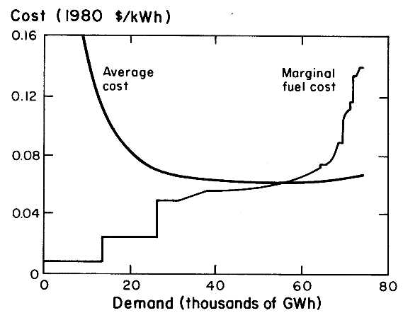
4.1. 1980 Marginal and average cost curves.
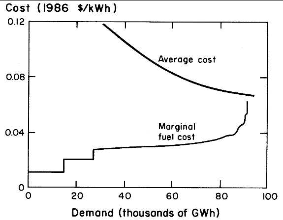
4.2. 1986 Marginal and average cost curves.
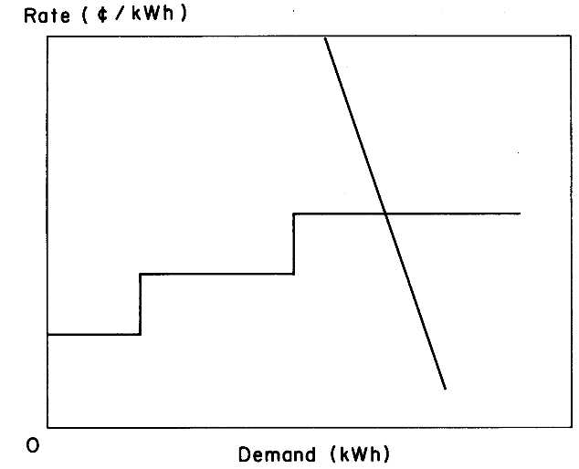
4.3. Tariff structure.
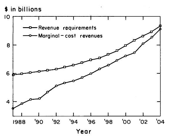
4.4. Revenue requirements and revenues from marginal-cost pricing.
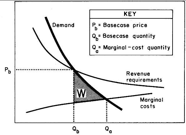
4.5. Economic gain from marginal-cost pricing.
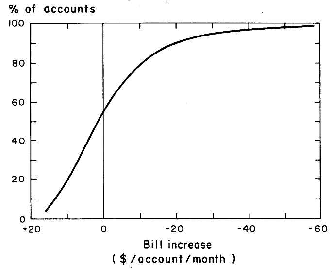
4.6. Impact of alternative rate structure: cumulative distribution (1987).
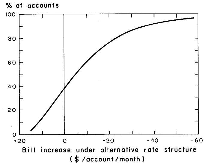
4.7. Alternative vs, CPUC rate structure.
FIVE
Natural Gas Distribution in California Regulation, Strategy, and Market Structure
Michael V. and David J. Teece
I. INTRODUCTION
Though stability has nearly returned to America's natural gas industry, the tumultuous events of the late 1970s and early 1980s will not soon be forgotten. The period's disruptive effects, manifested in swings in prices and supply, profoundly affected California's natural gas market. Among the reasons why a study of policy making during this unsettled time is instructive are the unique structure of the state's supply system, the political and social forces that historically have characterized statewide regulation, and the potential for this experience to lead to major change in future years.
This chapter focuses on the distribution segment of the industry in the years 1972-1986, a period marked at its beginning by the highest level of natural gas sales nationally and at its end by a new approach to regulating the state's gas market. The analysis spotlights California's two major gas distribution companies, Pacific Gas and Electric Company (PG&E) and Southern California Gas Company (SCG). Together, their retail sales accounted for roughly 95% of statewide sales in 1982.1
No study would be complete without an examination of the regulatory structure in which these companies operate. The principal agencies involved are the Federal Energy Regulatory Commission (FERC) and the California Public Utilities Commission (CPUC). This chapter will de-
scribe the elements of regulation as used in practice by these agencies, particularly the CPUC. Textbook models of regulation that assume continuity and instantaneous adjustment will be shown to be particularly unhelpful in trying to understand the realities of natural gas regulation in California. We will demonstrate how the gas market responded to the pursuit of sociopolitical goals established by regulators and to sudden and unpredicted economic change, and how the policies of utilities and regulators have greatly affected the California market. We will show how the regulatory process is characterized by strategic behavior by both utilities and regulators, and we will attempt to capture the ultimate effect of this contentiousness on economic welfare in California. We will also analyze the costs of gas distribution to gain insight into economic efficiency and cost minimization under regulation.
Special attention is directed to the industrial sector, which is one of four retail classes commonly identified in California. The others are residential, commercial, and electricity generation. Although the cost of serving industrial customers is undoubtedly less than most of the other classes, until recent years customers in this class paid substantially higher rates than the residential, electricity generation, and commercial classes. Because during the initial years of the study industrial users paid less than the average, at prices presumably closer to actual costs, the transition to higher relative prices was both rapid and painful.2
The overall goals of this study are to develop a deeper understanding of the California natural gas market and to provide the foundation for policies that will facilitate the transition to a competitive future. We will use a strong historical perspective to gain a depth of awareness with respect to current problems and opportunities. Section II will describe the federal regulation of natural gas prices and sales. The natural gas market in the state of California is the focus of Section III. Section IV will discuss California gas ratemaking during the study period, considering the issue of imbedded cost of service estimates developed by the CPUC and one firm it regulates. Section V will investigate that portion of the burner-tip price associated with transporting the gas from the utility's border (generally referred to as the city-gate) to its ultimate end use (generally referred to as the burner tip). A description of the response of industrial users to the present conditions then follows. Finally, we conclude with recommendations as to policies that can assist in the further transition to an economically sustainable California gas market.
II. THE NATIONAL MARKET
Historical Background
Gas was first put to commercial use for lighting city streets. It was not natural gas but coal gas. Although electricity had replaced gas as the prime source of municipal lighting by the late 19th century, a new market for gas was to emerge, as the early 20th century saw the invention of appliances that used gas for household purposes, first for cooking, then for water and space heating. By the late 1920s, pipeline technologies had been developed that allowed low-cost long-distance transportation of natural gas from the newly discovered fields in the south-central states to urban markets to the east, north, and west (Tussig and Barlow, 1984). A rapidly expanding natural gas industry resulted.
Before its recognition and use as a valuable resource, natural gas production was influenced by regulations put in place by states in regard to oil drilling. Oil and gas ownership has long been governed by the rule of capture, which effectively means that oil or gas belongs to the owner from whose well it emerges. Because petroleum deposits do not respect property lines, the discovery of oil on a parcel of land usually meant that nearby land owners had to begin production immediately or lose their right to claim a share of the deposit. States, fearful of the waste associated with these practices, controlled the extraction procedures a producer could employ, such as a limit on spacing of wells. These conservation laws made it easier for the states to inhibit the waste of gas, originally seen as an unwanted by-product of oil extraction. They also set a precedent for state regulation of local gas industries.
Although states had the power to regulate local rates charged by gas distribution companies, interstate transactions were free from regulation until 1938. The absence of interstate regulation meant that the downstream control exercised by state commissions could not significantly affect the price paid by utilities at the city gates, where ownership passed from the pipeline to the distribution utility. Not surprisingly, many interstate pipeline companies were highly profitable during this period.
The Natural Gas Act of 1938 resulted from a comprehensive Federal Trade Commission study and lively congressional debate. The act subjected interstate transmission of gas to Federal Power Commission (FPC) control. Transportation rates were to be "just and reasonable." In addition, no company could extend an interstate pipeline into a market already served by an existing pipeline without the prior consent of the FPC. Although the FPC could regulate field sales by a gas producer to a pipeline if the two companies were affiliated, the FPC took the position that it had no purview over a transaction between separate companies. This interpretational issue was the subject of a number of congressional
bills intended to explicitly exempt nonaffiliated sales from federal regulation, but for different reasons each was met with a presidential veto.3 The courts were thus left with the responsibility of interpreting the act, and the Supreme Court got its opportunity with the Phillips Petroleum case in 1954.4
In 1954 Phillips Petroleum Company, the largest independent natural gas producer, raised its wholesale rates to pipelines. These pipelines passed along the higher costs, but the ultimate consumers, which in this case were states and cities to the north, complained bitterly. The Federal Trade Commission declined to review the case, and it was taken to court. The Supreme Court ruled in favor of the plaintiffs, assigning the FPC dominion over wellhead gas pricing.5
The case-by-case approach to rate setting initially employed by the FPC became onerous, so in 1960 it divided the country into several rate areas, setting ceiling prices for gas in each.6 The only distinction within the areas was between "old" and "new" gas, where new gas was that discovered after 1960. Dissatisfaction with the operation of the gas industry under these controls led to further disaggregation of gas price categories. The cumbersome nature of ratemaking for the 23 geographic areas defined by the FPC led to the setting of a nationwide price in 1974 for gas discovered after 1973. This basic structure, which retained many of the various subcategories for gas discovered before 1973, remained in effect until the passage of the Natural Gas Policy Act of 1978.
The Natural Gas Policy Act of 1978
Passed amid widespread fear of gas shortages at prevailing, regulated prices, the NGPA was intended to stimulate the development of new sources by deregulating new and high-cost supplies. Old gas supplies dedicated to interstate commerce before the introduction of the NGPA in Congress were to remain regulated indefinitely. New gas, generally that developed after this introduction, remained regulated until January 1985 or July 1987, depending on the depth of the well. High-cost gas supplies produced from deep wells and other expensive sources after the enactment date were deregulated soon after the act's passage.
The act also gave the FERC, the successor agency to FPC, some power to control wellhead prices at sources destined for intrastate sales. A complicated set of rules controlled how interstate pipelines were to pass
along costs of new gas to industrial users and power plants.7 The intent of this provision was to equalize the Btu cost of distillate oil and natural gas used for boiler fuel.
Under the NGPA, the prospect for higher natural gas prices triggered exploration for new gas, but incentives to produce more old gas were weakened. Furthermore, the pipelines rolled in old gas with new and high-cost gas, so that prices to customers reflected the average cost rather than the marginal cost of gas. The NGPA thus inevitably caused distortions and inefficiencies (Braeutigam, 1981). However, because of the excess gas supply on hand on January 1, 1985, one anticipated effect of the NGPA never took place. That date passed without the sudden increase in price predicted by observers as late as 1982,8 although price controls on vast amounts of new gas were lifted.
Recent Federal Regulatory Issues
The statutes of the NGPA were designed in anticipation of continued escalation in energy prices. For the first several years, this expectation proved accurate. As just mentioned, some of these distortions and inefficiencies were predicted. However, the effect that the NGPA would have on the ensuing soft natural gas market was not widely foreseen.
A combination of several factors, notably increased competition from distillate oil, the effect of conservation efforts, and warmer-than-expected winters caused an ebb in the demand for gas, starting in late 1982. Gas pipelines found themselves without markets for their gas supplies, but bound by take-or-pay contracts to continue accepting or paying for gas.9 Estimates of the gas surplus vary, but the Department of Energy released figures in 1986 (Energy Information Administration, 1986) showing the surplus rising from 660 to 2036 billion cubic feet and staying at that high level through early 1986. During the post-1982 years, it became apparent that the NGPA offered little guidance when prices were in decline.
Previously, due to rolled-in pricing and the perception that gas prices would continue to climb, purchase prices for new and high-priced gas rose to record levels during the 1978-1982 period, topping out at over $11/thousand cubic feet.10 The tendency to pay well above the prevailing
market price for new gas supplies may have been affected by a given pipeline's endowment of old gas; the more old gas it had to "cushion" the cost of the new and high-priced gas it purchased and rolled in, the more it could afford to pay for this gas and still remain competitive.11 This strategy stemmed from the pipelines' expectation that a ready market for any gas existed, assuring the viability of rolled-in pricing. When the market softened, however, pressure on pipelines to curtail pipeline purchases of high-cost gas increased. The result has been the take-or-pay crisis, an important problem in the natural gas industry that will be addressed below.
In resolving take-or-pay liabilities and a host of other issues, the FERC has felt it necessary to balance equity and efficiency on several fronts. Consider the pressure exerted by end users and utilities to purchase gas directly from producers and pay pipelines only for transportation. Such contract carriage represents a more efficient option for end users and utilities because it reduces their costs. Unfortunately for the pipelines, gas purchased at levels too high to sell without rolling it in with lower-cost gas may remain unsold if the use of contract carriage broadens. Most of the commitments by pipelines to purchase high-cost gas reserves were made under a regulatory regime that assumed that parties at either end of the pipeline would never recontract. Therefore the issue of fairness to the pipelines became a salient one at the FERC. But the equity/efficiency trade-off also persists at the up- and downstream ends of the pipelines. Gas producers, who had installed facilities to extract higher-priced gas based on very favorable contracts with pipelines, and captive customers who have only one pipeline from which to purchase both complained bitterly (Stalon, 1986).
The FERC's early responses to these protests reflected the intent to phase in direct sales by producers to consumers. The FERC's Order 436 (Federal Energy Regulatory Commission, 1985) represented an attempt to respond to the needs of consumers by giving incentives to pipelines to offer contract carriage on a nondiscriminatory basis.12 Although there were allegations that pipelines did, in fact, discriminate, the program appears to have gained acceptance among pipelines (Wall Street Journal, 1986)· A second proposal is the so-called block-billing system. Under this program, gas would be separated into two blocks, essentially based on whether it was old gas (block 1) or new and high-cost gas (block
2). Block I gas would be allocated to each pipeline customer based on historical usage; needs beyond that level could be met in a variety of ways. These FERC initiatives represent efforts to bring prices in line with marginal costs in the industry, while respecting equity considerations by preventing discriminatory pricing to the extent possible under existing regulatory conditions.
It will be helpful to review the prospects for deregulation of wellhead pricing and pipeline transportation. Given the FERC's public statements concerning the remission of regulation in the natural gas industry,13 such an exercise is no longer academic.
Wellhead Deregulation
Under the NGPA, there is provision for deregulation of a majority of gas after 1985. By early 1985, gas purchased from price-controlled wells represented only about 36% of the total (Williams, 1985). One can expect that over the long run there will be some movement toward market-driven pricing in the industry, as supplies of indefinitely controlled old gas are depleted.14 Although proponents of decontrol can take some comfort in this prospect, the depletion argument understates the magnitude of remaining distortions because the NGPA stipulates that the price of additions to reserves of old gas be controlled. Thus one lingering inefficiency will remain: if additions to old gas reservoirs cost more to recover than their controlled price, they will remain in situ, even though their value on the spot market or in contracts may be well in excess of the cost of recovery. A study by the Office of Technology Assessment (1984) estimated the incremental effect of decontrolling old gas reserves, the sum of additions due to delayed abandonment, infill drilling, and well stimulation, at 19-38 trillion cubic feet. This number represents a 9.5 to 19.0% increase in the nation's gas reserves, as measured on January 1, 1984. Insofar as these incremental supplies are instead replaced by higher-cost supplies, wasteful expenditures are made.
As described above, the historical reason generally advanced for the institution of wellhead price regulation under the Phillips decision was the perceived market power wielded by upstream producers. Regardless of whether producers did, in fact, have market power at that time, our opinion, as Well as that of most observers, is that this is not the case today. This view is corroborated by a 1983 Department of Energy study (Energy Information Administration, 1983), which investigated seller concentration in major natural gas producing areas, each smaller than relevant markets. In no area of the country, except Alaska, did the own-
ership percentage of the 16 largest producers exceed 61.3%. Furthermore, aside from Alaska, no Herfindahl-Hirschman Index for any of the nine major areas15 was above 0.062, which, using the Department of Justice's criteria, makes each area "unconcentrated."
Thus on strictly economic efficiency terms, the argument for continued regulation of any gas reserves is weak. The preservation of this regulation can best be seen as politically motivated. As such, one can understand that the essential struggle is over the perceived benefits from regulation flowing to the various segments of the country's population. Evidence of the enormous importance attached by regional interests to the wellhead price deregulation issue is shown in a study by the National Regulatory Research Institute (1983). The study focused on 47 bills concerning the gas industry introduced into the House of Representatives in the first six months of 1983. Seventeen of these bills dealt with price controls.16 What one clearly sees in this analysis is that major differences among states, generally based on whether they produce or consume gas, drive the activity of their representatives in these matters. Producing states want deregulation; consuming states favor continued regulation.17 Given the different, and often conflicting, goals of politics and economics, this is not surprising, but it indicates the importance of leadership from the federal agencies, such as the FERC.
The impact of deregulation of wellhead prices depends in part, however, on the behavior of interstate pipelines and on the regulatory posture of the state regulatory commissions. The existence of any market power could impede the relay of marginal-cost pricing signals to final consumers.
Pipeline Deregulation Issues
To determine the feasibility of deregulation, a model to assess market power is needed. Analysis of oil pipelines (Teece, 1985) indicates that if workable competition exists in the relevant product markets, pipeline regulation is not needed. Some information on the relevance of this principle to interstate gas pipelines exists (German and Roland, 1985). Table 5.1 displays data on the number of pipelines serving producing
areas. These data indicate that the larger fields, representing 95% of total production, are, on average, served by a large number of pipelines. The table, however, aggregates data in a way that may distort the apparent competition, because not all gas in a given area can be obtained by any pipeline operating there.
When one considers the downstream end of interstate pipelines, the issue becomes more complex. Table 5.2 describes aspects of the resale market. This information is based on a sample of 26 companies developed by the American Gas Association (AGA). Although German and Roland conclude that 84% (58% + 26%) of sales are to distribution companies with alternative suppliers, the data do not accurately reflect the degree of competition, because the presence of just one alternative supplier need not always generate adequate gas-to-gas competition. In addition, of course, one would also like to be able to account for interfuel competition.
Further insight is provided by a separate AGA publication (American Gas Association, 1985), which disaggregates the first category. After deleting pipelines that provide less than 5% of a distribution company's need, the 58% figure shrinks to 53%, distributed as shown in Table 5.3. But these data are based on volumes, not points of transactions. According to Mead (1981, cited in Broadman, 1986), about 70% of all distributors are served by a single pipeline. For the remaining 30%, Broadman (pp. 18-19) points out that:
Even where distributors are served by more than one pipeline there is some question as to the technical feasibility of switching among suppliers. Some distribution companies have non-integrated supply systems which, in effect, segment the distribution network into two or more independent systems. More important, a pipeline's capacity at delivery points generally is tailored to meet a specific level of demand. In the short run, shifting the balance among pipeline-suppliers may well be constrained by limits on the physical capacity of one (or more) of the pipelines.
Unfortunately, simply counting interconnect possibilities is not a particularly good way to measure the state of competition that gas pipelines face, and further analysis is needed. This analysis should include the effect of competition in end markets, such as that from fuel oil and local gas producers.
Take-or-Pay Issues
One additional feature of the national gas market that should be mentioned involves the contracting practices of pipelines and producers. Along with the physical structure of the industry, regulation engendered unusual provisions in these contracts. Although once useful, the chang-
ing market for natural gas has undermined the viability of a number of these provisions and brought into question the enforceability of contractual commitments to purchase gas at the wellhead.
A number of provisions typically found in natural gas wellhead purchase agreements are peculiar and rather idiosyncratic to the natural gas industry. Virtually all contracts contain obligations for the purchaser to take a minimum amount of gas at the stipulated price. A number of methods for redressing the failure to draw such "minimum takes" have been used. The most popular is the so-called take-or-pay provision, wherein the pipeline agrees either to take a minimum amount of gas or pay for it as if it had. Pipelines generally can take delivery of the gas at later dates, but payment must be made in the specified period.
Masten and Crocker (1985) portray the take-or-pay stipulation as an efficiency mechanism that induces pipelines to refuse deliveries only at the point where an alternative purchaser would be willing to buy that gas. The level of gas the pipeline must take from the producer as a percentage of its total receivability varies with factors relating to the market structure of the gas field and the extent to which the price ceiling on that particular type of gas is binding. Masten and Crocker find that the take level varies directly with the number of sellers in a field and the free market value of the gas and inversely with the number of pipelines serving a field and their concentration.
Even though take-or-pay provisions may be rooted in the pursuit of economic efficiency, the extent to which pipelines exposed themselves to risk through these commitments indicates an industrywide bet that the gas market would not soften as it did. In fact, high demand for gas and continued shortages in the mid-1970s made the possibility of a gas surplus appear so remote to pipelines that they were willing, on average, to commit to take more than 80% of gas under contract to them.18 Conditions changed somewhat from 1979 through 1982, but even in 1982, no NGPA category of gas had an average take below 75.8 percent (Energy Information Administration 1982b).
However, when the nationwide surplus of gas developed, a number of major pipelines began incurring enormous liabilities. In 1983, six had accrued potential liabilities in excess ors 100 million (Energy Information Administration, 1986). In 1984, although over $3.6 billion of liabilities
had been settled, another $3.4 billion remained outstanding. That figure rose to $5.6 billion in 1985.19
These consequences have sent gas pipeline legal staffs searching for ways to justify their unilateral cancellation of major contracts. A number of legal doctrines theoretically could be drawn upon to legitimize these actions. One is claiming umbrage under force majeure clauses, the same provisions that protect companies against uncontrollable natural events, as well as labor strikes and well blowouts on occasion. Another possible route is using the doctrine of commercial impracticability, which has generally been used when an unforeseen event makes contractual performance economically unviable.20 Neither of these escape hatches, however, will necessarily lead to release of take-or-pay obligations for pipelines. The issue appears headed for the courts.
Future Federal Role in Natural Gas Regulation
A bold policy initiative would be to deregulate the entire natural gas industry upstream from the city gate immediately. Advocates of a more measured approach advance three reasons why caution should be exercised.
First, gas that is controlled in price is held so far below its market value that a sudden increase in its price would have major short-term ramifications. New, high gas prices, which have been inflated by rolled-in pricing, could collapse. The ensuing adjustment period could be quite severe.
Second, and related to the first, is the issue of long-term contracts. In the event of decontrol of old gas, pressure for abbrogation of contracts for new, high-cost gas will mount. As described above, most of the contracts for these supplies executed in the post-NGPA period do contain provisions to protect the producer if decontrolled new prices result in higher prices but do not correspondingly protect pipelines if decontrol of old gas suppresses new gas supplies. Thus there are asymmetries in the response of old and new gas prices under decontrol, indicating that prices could rise in the short run.21 Policymakers also have to consider this effect of deregulation before finalizing new rules in the gas industry.
Finally, although the data are not as conclusive as one could hope for, some analysts point to strong circumstantial evidence indicating that in-
terstate pipelines do possess some market power. To ensure that decontrol works properly, concurrent attention will have to be focused on pipelines to study the extent of this power. If market power has been present, we believe that Order 436 sufficiently addresses the situation. As more pipelines become "open" under 436, pipeline market power will be eliminated.
Thus the evidence surveyed in this section indicates that workable competition exists in wellhead markets, and it appears that decontrol of old gas prices would assist efficiency goals. For political reasons, contract carriage will probably need to accompany gas price decontrol to ensure that the benefits wellhead deregulation brings to consumers are not captured by upstream pipelines. If persistent evidence exists that nondiscriminatory voluntary carriage is being resisted by pipelines, the FERC might consider mandatory carriage as a solution. A more drastic policy would be to make pipelines common carriers.
We now turn our attention to positioning California in the national setting, with special emphasis on how the state would fare in a deregulated gas price regime.
California in the National Setting
The California natural gas market is large by national standards, accounting for 9.6% of the country's consumption in 1983 (American Gas Association, 1984). In addition, the prospect of an enormous new market for gas in Kern County ensures that California's role will be great in the foreseeable future. California is also a major market for Canadian gas, receiving 23% of that country's gas exports in the United States in 1982 (American Gas Association, 1984).
California is endowed with major in-state gas reserves. In 1982, it produced 385 billion cubic feet of gas, equal to about 13% of its consumption. California is one of only two states in which no in-state production enters interstate markets (Michigan is the other). Rather, whatever gas is not used by the owner is generally sold to the local distribution utilities. Because Canadian imports represent an additional 20% of the state's consumption,22 in 1982, gas not regulated by the federal government comprised about 33% of California's usage.
For in-state production, a classic monopsony situation applies, with the local utility acting as the sole available purchaser of gas. This situation, along with the low cost of transportation to the utility system, has kept in-state reserves relatively inexpensive. For PG&E, California gas was priced an average of 17.3% below PG&E's average for the years 1981 through 1985. On the other hand, the Canadian gas that PG&E
purchases has cost as much as 51% more than the system average price.23 This situation may be the result of the relative bargaining position at the time of the execution of the contract with Canada. In any case, the importance of long-term contracts is still very high; PG&E's minimum takes of gas from its suppliers represent about half of all of its purchased volumes.
It is difficult to assess the effect of gas price deregulation on California markets. Presumably, if a single (transportation-adjusted) price for gas then prevailed, old gas prices would rise, while new gas prices would fail. Complete decontrol of old gas, assuming that the market clearing price were stable, would thus result in an income transfer to states currently consuming large quantitites of new gas. Although the data do not permit one to trace from wellhead to burner tip exactly how much of a given state's gas purchases is old gas, an examination of the gas purchases of two of the pipelines accounting for a majority of the 56% of the gas coming to California from other states is instructive.
Table 5.4 gives information on gas purchases by the 25 largest interstate pipelines, as submitted to the FERC. These figures are based on the purchased gas adjustment (PGA) filings, made on a staggered basis from September 1984 through April 1985, representing purchases in the previous six months.
Even for the two California suppliers, the endowments of old gas differ considerably. For the sample as a whole, the range of percentage of reserves comprised by old gas runs from 3.7 to 64.7%. The weighted average cost of gas purchased by California's suppliers was more consistent, averaging $2.71 per thousand cubic feet, close to the national average.24 For the nationwide sample, this number ranged from $2.06 to $3.73, a considerable range.
These numbers seem to indicate that not just rolled-in pricing has varied the purchasing behavior by the pipelines. If this were so, one would expect a narrower range in weighted average purchase costs, regardless of the differing endowments of old and new gas. The range of purchased costs may also provide a reason why pipelines may be resisting the more competitive environment that contract carriage would engender; given these figures, high-cost pipelines would have difficulty marketing their own supplies.
Because California appears to be near the median in terms of both old gas endowment and average costs, decontrol would probably not cause severe adjustment problems, assuming prices for higher-priced
gas are free to decline so that a market clearing price is sustained.25 Also, because California receives large quantities from in-state and Canadian sources, the impact of any sudden increase in interstate costs would be softened somewhat.26 We should point out that the lack of crucial data, such as the exact nature of contract provisions and of the makeup of gas reaching California from interstate pipelines, makes this analysis necessarily speculative.
As stated above, without pipeline contract carriage requirements being linked to further (or full) wellhead decontrol, the effect of price decontrol at the wellhead is uncertain. In the absence of contract carriage there is some chance that gas pipelines would be among the beneficiaries due to the concentration of interstate pipelines serving California.27 Whether California consumers would lose from wellhead deregulation in the short run will depend on whether market and environmental conditions permit competition from fuel oil. In the long run, we expect that welfare gains from gas field decontrol will outweigh any short-run losses.
III. NATURAL GAS IN THE STATE OF CALIFORNIA
The purpose of this section is to provide background on the nature of the market for natural gas in California. We will examine gas distribution companies, the state regulatory agency, and retail gas customers, particularly those in the industrial sector.
California's Major Gas Distributors
Figure 5.1 shows the system of gas pipelines operating in and around California. Several large mains that originate in the Texas gas fields enter the state. The major lines are operated by the El Paso Company and Transwestern Pipeline Company. The former is a subsidiary of Burlington Northern, Inc., the latter of Houston Natural Gas Corporation. To the north, a large pipeline operated by Pacific Gas Transmission
Company, a subsidiary of PG&E, brings gas from the western provinces of Canada to California. The network of smaller lines in northern California represents the Sacramento Valley gas fields; the southern network represents those of the San Joaquin valley. Figure 5.2 shows service areas of the two main gas distribution companies in the state.
Table 5.5 shows how the supplier profiles of PG&E and SCG have changed by contrasting their gas sources for 1982 and 1986. Although Canadian supplies have remained its largest source, PG&E has reduced its purchase of higher-cost El Paso gas by over one-half, substituting it with spot purchases. After making its first spot purchase in 1985, PG&E has strikingly expanded the role of these spot markets. California and Rocky Mountain purchases remained steady. PG&E serves most of northern California. Of its total load, approximately 71% is sold to residential, commercial, and industrial customers; the rest is used for electricity generation (Table 5.6). These electricity generation requirements account for a large portion of the gas company's revenues, reflecting the resource mix of the PG&E electric utility, which depends heavily on fossil fuels.
SCG serves most of southern California. Like PG&E, it has reduced purchases from southwestern pipelines by about one-half and sharply increased its use of spot markets (Table 5.5). It has also increased its use of Canadian and California onshore producers and greatly expanded its purchases from offshore sources and PG&E (mainly the former source). Unlike PG&E, it is not integrated into power production, so it sells a large quantity of gas to electric utilities for power generation. It also provides the City of Long Beach and San Diego Gas & Electric Company with their natural gas needs. The latter transactions are termed sales for resale or wholesale sales and comprise approximately 14.5% of the gas sold annually. The majority of gas is sold to customer classes as shown in Table 5.6.
Sales to customers are made according to several different price schedules, which correspond to priorities set by the CPUC, as well as according to whether or not the supply is delivered on an interruptible basis. There is a lifeline allowance for residential users, which differs by location within the system, home heating equipment (gas or electric), and time of year. In this chapter, we will often use a classwide average to describe customer rates for simplicity.28
Figure 5.3 shows the delivery profile for PG&E in 1984; SCG's is similar. Because gas can be stored for future use (usually underground in natural reservoirs), the utility has the ability to "bank" gas for later use. Fortunately, California's gas demand exhibits seasonal complementarities. Residential gas demand peaks during the winter, while utility gas demand peaks during the summer (generally the late summer, when hydroelectric resources are depleted). By using storage, the utilities are able to keep their gas demand at a nearly constant level, though it still peaks in the winter. Because their suppliers base part of the gas charge on the peak level of gas delivered to utilities, storage helps to moderate overall gas costs.
In contrast to most other states, no interstate pipelines pierce the state's borders, giving California gas utilities complete control over out-of-state gas sales in California. The gas line that brings Canadian gas to California terminates one foot from the border, where ownership is transferred from Pacific Gas Transmission Company to PG&E. Thus the FERC, which regulates gas destined for interstate sales, has no purview whatever within California.29 Instead, the CPUC has almost complete control over rates, a powerful position that has been well exercised.
The California Public Utilities Commission
The CPUC exerts authority over a number of state industries, from telecommunications to commuter railroads. It has achieved a national reputation for technical expertise, regulatory zeal, and the willingness to experiment with new programs and technologies. Working with utilities, it has developed a number of progressive approaches to conservation. It also has been involved in soliciting private electricity generation in California. The CPUC has always championed low prices for consumers, and in 1976 it acted on a legislative mandate to set a lifeline allowance for residential customers.30 After 1977, when appointees of Governor Jerry Brown achieved a majority on the commission, it increasingly pursued social goals, a thrust that more often than not translated into cross-subsidization of residential consumers by commercial and industrial classes. It also adopted several policies that have allowed certain price signals to reach the consumer sooner than otherwise. For instance, it instituted an adjustment mechanism in 1973 that allows utilities to raise or lower rates automatically every three months to account for
changes in fuel costs. Current policies, described below, allow larger customers to recontract periodically for utility gas, in direct competition with other suppliers.
Ratemaking with respect to general rates takes place on a three-year cycle in California.31 The rate base is generally set in accordance with the principles of original cost. Until 1987 rate design had ostensibly been based on value-of-service pricing, although this terminology had never been precisely defined by the commission. As practiced, value-of service pricing is distinct from Ramsey pricing, with which it is often confused. Under Ramsey pricing, the ratio of the markups over marginal costs for two customer classes is set equal to the inverse of the ratio of their elasticities. Thus, the higher a class's elasticity, the lower its relative price.32
Under value-of-service pricing, prices are set in proportion to willingness to pay for a particular good or service. The important point is that willingness to pay is not necessarily equal to the inverse of a customer's elasticity. The assumptions employed by the Commission in choosing prices were that industrial and commercial customers had a higher willingness to pay than residential customers. In the case of industrial customers, the use of a willingness-to-pay criterion rather than the use of elasticity measures meant that their prices exceeded those of the residential sector. Under a Ramsey pricing regime, the industrial market would have received gas at the lowest prices because it is the most elastic.
Gas Utility Customer Classes
Residential customers form the largest component of demand for natural gas in California. Collectively, they purchase more cubic feet of gas than the industrial and commercial classes combined. It is residential customers who historically have been the recipient of cross-subsidies authorized by the CPUC. In part, this may have been due to their captive position. Unlike an industrial or electricity generation customer who can exercise some interfuel substitution if the price is right, residential customers have only conservation as a ready alternative.
Commercial classes fared the worst under value-of-service pricing. They experienced frequent rate increases, under the presumption that their willingness to pay was high. They have been squeezed even tighter in recent years, as pressure from the industrial sector has resulted in re-
lief for that class. In some cases, it was cost-effective for commercial customers to burn propane rather than natural gas. The main problem may be that, unlike other users, the commercial users have not yet developed any effective means for regulatory plea bargaining.33
Industrial customers have been in a very different situation from commercial customers. Historically, they have switched from natural gas to fuel oil based on economic conditions. Table 5.7, which displays California data, shows that industrial consumers do exhibit sensitivity to the relative price of gas and oil. Since 1982, regulations have prohibited the combustion of Nos. 5 and 6 fuel oil in industrial boilers, the reason later years are omitted. The figures indicate that a large number of users either cannot purchase fuel or have transportation costs that make oil use cost-ineffective, even given the average numbers above. The figures show that industrial customers do respond to changes in the relative prices of competing fuels, the correlation coefficient between the price ratio and gas sales being-0.658.34
Given the cleaner-burning characteristics of gas, state regulatory authorities have been reluctant to implement policies that would facilitate switching away from gas. This policy preference has, at times, clashed with federal regulation, notably in the case of the Power Plant and Industrial Fuel Use Act of 1978 (PIFUA). The act was passed to encourage the use of coal and synthetic fuels by large users, with the expectation that both sources would expand rapidly in coming years. Although this aim was understandable in the face of the expectations of dwindling natural gas supplies at the time of passage, the result in markets in which the primary choice is between oil and gas was to promote oil combustion implicitly.
The demand for gas for electricity generation by utilities forms a most interesting market segment. It is in this sector that the two major distributors differ. For PG&E and SCG, gas sales for utility electricity generation constitute internal and external transactions, respectively. Later sections will show that sales to gas-fired power plants, a major competitive nexus between electric and gas services in California, have been used strategically by both the utilities and the CPUC.
IV. THE VALUE-OF-SERVICE EXPERIENCE
This portion of the chapter evaluates the value-of-service structure employed by the CPUC until 1987. Our aim is to show how this pricing was used to pursue a number of social goals, how the CPUC grasped the opportunity, and how the distortions it created ultimately resulted in its abandonment. We discuss the historical background of value-of-service pricing, consider an interesting case concerning the problems with determining actual costs of service, and conclude with a description of the new direction of gas regulation in California.
Historical Background
We will investigate the setting and designing of gas rates by the CPUC in this section, drawing extensively on statistical information for PG&E and SCG. Figure 5.4 shows the historical trend of delivered gas prices for the retail classes for PG&E; the trends are very similar for SCG. With a few exceptions, the trend is monotonically upward. Although this course reflects the general rise in natural gas prices, a closer inspection reveals that the four retail classes—residential, commercial, industrial, and electricity generation—have fared differently from 1972 to 1985.
Before 1974, ratemaking was based on the principles of cost of service, so that residential and commercial customers paid rates in excess of the average retail rate, reflecting the fact that the provision of service to them was more costly. Beginning in 1975, rates began to move toward equality across the various classes, although ostensibly no change in ratemaking policy occurred. This movement may have been induced by consumer pressures, caused by the onset of higher energy prices in 1974. In 1977, however, the ascendancy of the Brown administration appointees to a majority in the CPUC, the prospect of severe gas shortages, and the legislative directing to establish baseline rates led to the formal adoption of value-of-service rates.
This method of designing rates can be used to keep total utility revenues at acceptable levels, given steady or declining sales. Prices arc set based on willingness to pay, and for ratemaking purposes the CPUC placed industrial and commercial classes higher on this scale. In California this meant raising industrial and commercial rates substantially more than residential rates. Industrial rates (until 1984) and commercial rates have risen markedly with respect to average rates, while residential rates have declined. Electricity generation prices under value-of-service also rose. This growing cross-subsidy, which would be even more pronounced if actual cost-of-service figures were used rather than average retail rates, prompted increasing resistance from commercial and industrial customers. The cost-price distortion, as will be shown, had major structural ramifications in the industrial sector.
But these cost-price gaps were necessary to comply with the directives of the state legislature to suppress residential rates. In 1975, after several years of rapid gas cost escalation, legislation was passed calling for the CPUC to reconstitute gas rates so that the first portion of residential therms were priced under the residential class average. These new rates, now known as baseline rates, call for this allowance to be priced at 85% of the class average.35 This policy forced the CPUC to make up these revenues elsewhere, a major factor contributing to its adoption of value-of-service pricing.
Even if the assumptions regarding the willingness of the various customer classes to pay were accurate, value-of-service rate design policies have drawbacks. Because gas faces interfuel competition, tariffs so determined for industrial users were no longer sustainable. As we shall see, this practice induced severe market distortions, such as "cream-skimming" entry in customer segments that provide high-margin contributions. In deciding to return to a rate design based on cost of service, other serious consequences may develop.
Abandoning value-of-service pricing involved several problems for the CPUC. There are a number of political and strategic reasons why the commission found that pricing structure attractive. Perhaps the most important is that it guaranteed the agency broad discretion in setting rates, because the key allocational tool, the relative willingness of the various classes to pay, could not be objectively and definitively determined. The CPUC, therefore, was free to adjust rates as it saw fit, as long as the total revenue received by a utility is held constant. In several cases, this discretion led to the reconfiguration of rates within various classes, to prevent oil combustion or to pursue political goals.
In the case of pricing natural gas to industrial customers capable of switching from natural gas to oil, the CPUC priced gas to these users in a way that precluded the combustion of residual oil. The policy involved calculating a proxy value for delivered oil and then setting the gas rate just below this value. To arrive at this value, the commission started with the price of Indonesian low-sulfur waxy residual oil, then added a factor for taxes and transportation to the ultimate consumers. This constituted a form of limit pricing, characterized by the posting of a price designed to deter entry by a competitor.
Not surprisingly, the combination of lags in rate setting during periods of falling oil prices and regional differences in actual oil transportation charges among industrial customers has meant that some oil, nonetheless, is burned for industrial purposes. In a more subtle vein, the difference in rates between industrial customers with and without boilers
fitted for dual fuel combustion widened considerably during the early 1980s. Those customers without the capability to switch fuels were charged much higher rates (28% in the PG&E service area in 1984). The artificiality of this gap from a cost-of-service perspective is underscored by the fact that there is little basis to claim a difference in that cost between these two customer groups.
One fascinating example of the political factor in ratemaking as formerly practiced by the CPUC centers on the pricing of gas destined for use in electricity generating plants across California. These sales are made in a clearly identifiable transaction by SCG to Southern California Edison Company (SCE); for PG&E they represent an internal sale from the gas side to the electric side of the same company. Sales for electricity generation by both SCG and PG&E's gas side have presumably been held well above costs of service because of the CPUC value-of-service policies.36
Another reason why electricity generation rates have been held high is the set of social goals that the CPUC emphasized. Among these goals is the support for private electric power generation. According to the statutes of the Public Utility Regulatory Policies Act of 1978 (PURPA), electric utilities are required to purchase electricity generated at privately financed facilities, provided that this electricity is produced at qualifying facilities, defined as those using renewable or cogeneration technologies. The price paid by utilities per kilowatthour is to be its full avoided cost, that is, the savings to the utility for not having to produce that same kilowatthour of electricity itself. The typical California electric utility would have produced a kilowatthour on the margin during a large portion of the summer months by burning natural gas.37 For this reason, the higher the purchase price of gas to the utility during this period, the higher the price paid to private power producers.
Because of the CPUC's strong support for the concept of small power production, it kept the gas price to electric utilities at levels that meant
a major incentive for qualifying-facility development in California. The policy has also had the effect of generating revenue to help keep the increase in residential gas rates relatively low as gas sales for electricity generation provided a source of cross-subsidies to gas recipient classes. However, in 1984 the CPUC began to recognize this pricing distortion, stating that in PG&E's case, the "[electricity generation] rate is out of touch with today's fuel markets" (California Public Utilities Commission, 1984, p. 76). In its 1986 decision discussed below, the CPUC decided to treat electricity generation loads as identical to large industrial loads and price accordingly.
The responses of the electric utilities to this policy shed light on the complex intertwining nature of ratemaking. In California, as elsewhere, new power plants are subject to a prudency review before being allowed into a utility's rate base. A crucial part of this review is the comparison of the fuel savings to the company to the cost of the new plant. Thus the higher the current and projected marginal-cost savings to the utility, the better a new plant looks economically. Because both PG&E and SCE have newly completed nuclear units, both targets of accusations of managerial bungling, they are anxious to have the specific question of economic need for the plants resolved. The ex post facto nature of this review certainly is open to criticism, but such examinations have become the rule for regulatory commissions. Because the marginal costs saved by its new nuclear plant (and projections for future savings) are strongly influenced by the price its electric side "pays" its gas side for gas supplies, until recently PG&E did not protest this price with much vigor.
Another possible reason for PG&E's acquiescence to the policy of maintaining a high electricity-to-gas transfer price was that it gave the company the opportunity to offer lower rates to industrial customers, including those able to switch from the SCG system to PG&E's. SCG could not respond directly to this challenge for two reasons. First, its electricity generation sales represent a real, external transaction. Second, SCE protested to the CPUC about the high price it was being charged by SCG for this gas. SCE, perhaps less concerned about the economics of its nuclear unit, threatened to begin widespread use of oil in its thermal plants as oil converged in price with gas. The CPUC responded by adopting an electricity generation gas rate schedule, which reduced SCE's gas rate, but only when air quality conditions allowed the burning of fuel oil. A much higher price is charged during episode days, when oil could not be used. The net result was a price decrease in SCE's gas bills.
Contemplating the Costs of Service
Our criticisms of value-of-service pricing should not be construed as implying that true costs of service can be determined unambiguously and
uncontroversially. A clear example of how differently the CPUC and a company can compute the relative cost of serving various customer classes is illustrated in 1985 studies by the CPUC and SCG (California Public Utilities Commission, 1985a; Southern California Gas Company, 1985b). Table 5.8 shows the average imbedded costs of service for four retail classes and combined wholesale classes for SCG. Although these numbers represent imbedded costs, they are based on historical costs and so do not necessarily correspond to economic costs.38
The actual numbers represent rates in effect at the time of the studies, adjusted slightly for comparability.39 SCG and CPUC calculations cover the 12 months beginning May 1, 1985, and are based on the same revenue requirement as the actual rates. The CPUC costs were developed using work papers supporting the analysis of the Public Staff Division (PSD). It should be pointed out that these figures do not necessarily represent the opinion of the CPUC as a whole. As such, they will be referred to as the PSD figures.40 To keep the fine-class breakdown, assumptions regarding the rate structure below were made.41 Also, the estimates were adjusted so that each corresponds to a purchased gas cost of $3.755/thousand cubic feet. Finally, each estimate would result in SCG meeting its nongas revenue requirement. The figures do not include the effect of regulatory balancing accounts. The differences between SCG and the PSD are illustrated in Figure 5.5. This figure summarizes very detailed and complicated allocation procedures used by both entities. These procedures are necessary to apportion costs other than that of gas, such as labor, new construction, and depreciation of existing infrastructure. The simplest allocation method is to add up all the
nongas charges and spread them equally across all cubic feet of gas sold. This "commoditizing" process is the most straightforward way to allocate truly common costs.
The major proximate difference between the two approaches is that of the total nongas charges; each assumes its own estimate of how much of these nongas charges are common costs. The PSD figures allocate roughly 67% as common costs, whereas for SCG this share is 8%. Other costs are allocated according to formulas using peak and average demand, cold and average year sales, or direct cost-based allocations. Ostensibly, the PSD assumed that SCG's allocation procedures for apportioning common costs to customer classes were based on specific formulas. The PSD contended that commoditizing a major portion of the nongas margin constituted a more accurate and fair approach in the absence of more precise knowledge.
In some instances, the PSD approach is appropriate. In other instances, such as when part of the SCG distribution system operation and maintenance costs are allocated to wholesale customers, it is flawed. Although it is difficult to endorse either approach, there is no doubt that the PSD figures buttressed the CPUC's value-of-service rate structure. By placing so many nongas costs into the jointly allocated category, the PSD study flattens cost-of-service estimates across the various classes compared with the SCG figures. For this reason, cross-subsidy estimates based on the PSD cost estimates are lower than SCG figures. The SCG estimates supported that company's claim that there were major pricing distortions under value of service.
For the purposes of this study, an analysis comparing 1985 rates charged SCG customers to PSD and SCG cost estimates was conducted. Figure 5.6 displays the total cross-subsidies received or contributed by class and represents the cost per thousand cubic feet multiplied by total sales to that class.
Looking at Figure 5.6, the difference in conclusions concerning residential customers is startling. That class received a small subsidy according to PSD cost estimates, but for SCG, this subsidy swells to $337.0 million annually. If sales by PG&E and smaller utilities were supported by the same amount per cubic foot as SCG residential sales, a statewide estimate of the total subsidy to residential customers in 1985 would be in the neighborhood of $600 to $700 million per year. Both PSD and SCG agree that commercial customers supplied major revenues, $171.6 million and $137.5 million, respectively. For industrial customers, both estimates show that this class also provided net revenues, but the two figures vary, placed at $55.5 million by PSD and $126.5 million by SCG. Interestingly, the conclusion concerning the electricity generation class differs, depending on whose estimates are used. For PSD, the class
receives a $133.9 million subsidy; for SCG, the class provides a $85.1 million contribution. Finally, although SCG cost figures set wholesale rates nearly at their cost, PSD cost figures show that wholesale customers receive $80.2 million annually from the SCG system.
The public policy implications of analyses based on the two estimates of cost are completely different. If one believes the PSD, residential customers have paid their way under value of service. The major subsidy ran from commercial users to the electricity generation and wholesale classes. If marginal rates were used, most of the subsidy to the electricity generation class would probably dissolve. However, the result that wholesale customers receive a major subsidy appears to be the result of the commoditizing of nongas costs, which perhaps should have been spread across the four retail classes, not all five classes. In any case, cross-subsidy figures based on PSD costs show that the value-of-service pricing system was much closer to one founded on costs than the SCG costs.
The SCG cross-subsidies show that residential customers were the recipients of huge benefits under this system, receiving about $100 to $130 million from each of the commercial, industrial, and electricity generation segments. This scenario appears to fit more closely with the outcome one would expect from a value-of-service format that assumes that residential customers are the least willing to pay for gas. The electricity generation subsidy, following the same logic as above, probably is much larger than the figures suggest. Most important, one can more easily see the impetus for entry into the industrial market. Entry by third parties was invited if they could price between current rates and imbedded costs.42 As we discuss below, the threat of entry by dedicated pipelines has become a central issue in the California regulatory arena.
Above all, what this analysis demonstrates is that there is a tremendous degree of gamesmanship involved in the California regulatory process. The analysis confirms the observations of Owen and Braeutigam (1978) in regard to the strategic use of the administrative process and suggests that regulators are not strangers to the use of gaming apparatus. Furthermore, an assertion that rates should be based on the costs of service, implying that these costs are precisely determinate, carries an unsupportable assumption. Indeed, considerable factual reinforcement exists for each cost structure studied here. The supporting documents for both sets of figures (as if to discourage validation efforts) present the dispassionate analyst with a considerable tangle of details. At this point, given the new move to prices based closer to costs, a common costing methodology is compulsory.
It appears that the need for good estimates for the actual costs of service is a concern in most of the industries regulated as public utilities; the CPUC itself has made the determination of these costs a major priority in a study of the telecommunications industry (California Public Utilities Commission, 1985b). Given the threat of entry in California industrial gas markets, precise knowledge about the costs of service would be an invaluable policy tool for the gas industry as well.
The New Direction of California Natural Gas Regulation
Responding to an industrywide clamor for regulatory reform, the CPUC initiated an effort to restructure gas rates in 1985. At that time, although it adopted methods to make contract carriage easier for large users, the CPUC recognized that a more fundamental and broader recon-figuration was necessary. After a year of extensive study and numerous hearings, it issued new guidelines which became effective on January 1, 1987 (California Public Utilities Commission, 1986a, b).
At the heart of the plan is the explicit acknowledgment of the dual nature of California's gas market. The main division is between those customers who can and cannot switch between fuels, although it is defined in terms of service priorities. The two basic consumer sectors are referred to as core and noncore, where the latter class includes fuel switchers.43 Within each sector are separate charges categorized as transportation and gas costs. Transportation tariffs are based on a formula that allocates each of the nongas charges between the core and noncore sectors using allocational techniques determined by the CPUC. These techniques recognize that both sectors should pay for existing infrastructure and demand charges, not just those customers who are captives of the utility. However, core customers do bear a larger portion of the cost burden, reflecting their higher service priority.
For the noncore sector, burner-tip gas rates will be determined individually because the CPUC has now allowed the utilities to individually negotiate transportation tariffs. The lowest tariff, based on short-run marginal cost estimates, is about 10¢thousand cubic feet. The highest, based on a proxy for long-run costs, is about $1/thousand cubic feet. This provision allows noncore customers to negotiate for a level of transmission security commensurate with their needs. It also allows utilities to conduct auctions for scarce capacity. Under additional provisions of the new rate structure, customers switching completely away from gas will still have to pay stand-by charges to the utility, corresponding to the cost of having that ready alternative.
Gas procurement for the two sectors also varies. Procurement of gas for the core sector will be made with high supply security in mind. As
such, it is expected to be more expensive and consist predominantly of long-term supplies, although the CPUC ordered the utilities to include some short-term and spot supplies in the core portfolio. For noncore customers, gas procurement will be made on a best-efforts basis, and supplies will be of a more short-term quality, so that prices will track national averages more closely. The obligation of the utility to serve non-core customers has been attenuated. In the case of gas procured by the utility for both noncore and core customers, the price will be the weighted average of the sector's portfolio. Thus even though transportation tariffs for noncore customers can be individually negotiated, gas commodity prices cannot. The adjustment mechanism by which fuel costs are included in rates will also be phased out for noncore customers.
The rules invite the noncore customers to seek out and contract for gas from other sources, paying the utility only for transportation. Large commercial customers in the core sector also have this option, although they must pay fixed transportation charges. Noncore customers can elect to receive gas from the core portfolio, although they can only switch back to noncore status when the noncore gas cost exceeds the core gas cost. However, these elected-core customers are subject to minimum billing, to ensure that they do not use core status to guarantee gas availability for large purchases made at infrequent intervals. This practice would have imposed the cost of insuring suppliability on other core customers.
On balance, the new guidelines are a giant step in the right direction. As we have argued, the natural gas distribution industry in California consists of not one but several markets, divided according to the nature of substitutability for gas. As now regulated, the particular needs of each market are better addressed. Except for residential and other small customers, transportation and gas services have been unbundled. Utilities are put under pressure to reduce their purchased gas costs, so as to retain the maximum number of customers for transmission plus gas. Industrial customers are free to cut their own deals if they are dissatisfied with utility gas; they are also free to suffer the consequences of poor decisions they may make. And costs are more properly borne by core customers for whom security of supply is a major priority.
There are possible problems that may have to be addressed. Utilities may view the ability to negotiate transmission tariffs as a license to price discriminate. Although discriminatory pricing has a long regulatory history, the ability to discriminate customer by customer is new to gas distribution. There will likely be complaints from customers who feel they have received unfair treatment, and the CPUC will have to decide how to deal with that issue. However, the competition to serve customers in the noncore sector is best addressed by allowing flexibility, not limiting
it. The new rules may also have the effect of directing the lowest cost supplies to the largest customers, which has angered consumer groups. Large customers may get the cheapest supplies now, but the situation could reverse if increased demand causes marginal rates to rise. But the retention of these customers on the utility rolls is important; they make positive contributions to the recovery of the utility's fixed costs.
Twenty-two parties, ranging from the interstate pipelines serving California to industrial user groups, filed comments and participated in the proceedings leading to the formation and adoption of the CPUC's guidelines. Under these contentious conditions, it is a positive sign that progressive results were obtained. The regulatory approach taken appears well suited to the need and the responsibility of the large industry players to control their own destiny. As the system is fine-tuned, we hope it will further enhance the efficiency of gas distribution in the state.
V. ARE DISTRIBUTION COSTS EXCESSIVE?
Background
In the preceding discussion of the divergence of cost and price in the California natural gas market, we pointed out that this growing separation led to markedly increased prices over time for some classes. Another historical cost trend in California has received less attention. It is a tendency that has taken place within the utilities themselves, and its effect has been to raise rates for all users. The issue is organizational efficiency.
X-Efficiency is a term coined by Leibenstein (1966) to describe the sources of efficiency that are not captured in neoclassical economic theory, such as motivational and institutional factors. X-Inefficiency refers to firm behavior that is non-cost minimizing, often attributed to a lack of competition. The idea that monopolies, either regulated or unregulated, could display X-Inefficiency has many supporters.
If X-Inefficiency exists in the natural gas distribution industry, one would expect that the market would result in distribution margins larger than competitive levels. One would expect a system displaying greater X-Ineffiency over time to display higher employment and salary growth than that of comparable competitive firms. This section will explore these issues by studying the employee component of distribution (or gross) margins. The gross margin includes depreciation and return on plant, operating, and maintenance expenses; administrative costs; and other constituent costs. Labor comprises the major portion of most of these items.
An unfortunate fact is that the data necessary to prove relationships convincingly are not publicly available, due to a number of factors.
Isolating the direct effect of being sheltered from competition on employee growth is difficult. The nature of work differs across utilities, but more important, growth rates during the period under study have varied widely between different geographic sections of the country. One should not expect employment growth within California utilities to equal that of utilities located in the Northeast or even the country as a whole. The spatial organization of service territories varies also. Population densities vary widely.
For these reasons, the analysis of employee growth will be conducted in a less rigorous manner than the analysis of salary growth, although the study of the latter variable is troublesome as well. The main difficulty associated with the study of salary structure here is that only company-wide average salary data are available. Previous studies of several other utility industries (Hendricks, 1975; Weiss, 1966) have isolated salary by job classification, possible with the use of census data. This allowed direct comparison of wages in regulated industries to wages in unregulated manufacturing industries. Unfortunately, because census data by job classification is available for industries only up to three-digit Standard Industrial Classification code level, only certain regulated industries, such as electric power production, can be analyzed in this way. Because the relevant data for gas distribution companies and transmission companies is aggregated, there is no simple way to obtain salary information by job classification for gas distribution companies. However, a study looking at the effect of differing competitive environments on average company salaries is interesting and will be developed below. A somewhat circumstantial but nonetheless arguable case that inefficiencies exist will be constructed. We will begin our study of distribution margins at the California state level.
Historical Trends
Focusing on the California utilities, the social and political objectives pursued by the CPUC in the past clearly affected how the total gross margin has been allocated among the consumer classes. The gross margins for the utilities in the years 1972 through 1985, calculated as the difference between the ultimate sales price for the customer class less the average utility gas cost (city-gate cost), rose for all classes. However, for customer classes that have suffered the greatest price increases, such as the commercial class, the margin has risen at a more rapid rate. For residential customers, the margin increase has been moderated. To get an idea of whether this increase in margins is unusual, a comparison of California rates to national averages from 1972 to 1984 was made to national averages. The results appear in Table 5.9.
The greater increase in city-gate (CG) prices experienced by the California utilities is likely the result of their commitments to purchase gas at later dates than the typical gas utility. Many of these commitments call for gas to be purchased at new gas prices, higher than average gas prices.
Table 5.9 shows that distribution margins (M) increased enormously compared with national figures. Considering average annual percentage changes, this difference in overall increases appears to be rooted in the years from 1976 to 1980. During this period, while the national average margin grew at 4.02%, the corresponding figures for SCG and PG&E were 13.42% and 18.82%, respectively. This phenomenon appears to be the result mainly of growth in customers and employees, both of which outpaced the national growth rate. The period from 1976 to 1980 brought major construction inflation, and the inclusion of considerable new capital expenses into the rate base by both utilities no doubt contributed to the higher distribution margin for each. The difference between the SCG and PG&E margin growth figures may be the direct effect of the difference in sales between the two companies. For SCG, major sales gains allowed it to spread its fixed costs across more sales units than PG&E, which experienced a sales loss.
In the 12 years from 1972 through 1984, PG&E's sales per customer declined by 47%; SCG's corresponding decline was very close to the national figure of 33%. This change probably reflects the migration of industrial users from the system, customers who shouldered a large portion of the total gross margin. The much greater loss of sales by PG&E certainly resulted in proportionately more fixed costs being added to each sales unit in later years than SCG.
Although employee increases at SCG far outstripped the national figures, this may be the result of construction operations. The PG&E employment figures are puzzling. Their apparent decline may be the result of the company's use of a central construction department for both gas and electric operations.44 For both SCG and PG&E, responding to CPUC mandates to pursue conservation and other demand-side approaches to controlling gas loads also influenced employee growth. In sum, it is difficult to make a conclusive case from these numbers either that employee growth has been excessive or that it has been appropriate. In the case of gas distribution salaries, a cross-sectional analysis can support more confident conclusions.
Wage Rates
Of the distribution margin, the share represented by labor costs, including overheads, is approximately 39%.45 Thus the relative salary structure is a major determinant of the level of that margin. This section will test the hypothesis that the varying competitive conditions experienced by gas companies affect their salary structure.
Whether labor unions are able to extract premium wages from regulated utilities is an important issue, with a long history of economic inquiry. A recent installment in the ongoing debate on the subject of market power, unions, and wage rates has been provided by M. A. Salinger (1984). Employing a careful statistical analysis, Salinger finds that "the combination of concentration and entry barriers allows firms to raise price above cost and that the primary beneficiaries of the monopoly power are unionized workers" (p. 167). Extending this result to regulated utilities is not as simple as it may appear. Depending on the nature of regulation, the firm may be prevented from expanding wage rates. Furthermore, comparing salaries in regulated and unregulated firms is fraught with difficulty. For example, Weiss (1966) hypothesizes that regulated firms may obtain higher-quality labor.
Hendricks (1977) conducted an extensive investigation of wage rates in regulated utilities. In his analysis, salaries for similar jobs in regulated and manufacturing industries are compared. Because wages are not significantly higher for workers in regulated industries, he concludes that there is little evidence that economic rents are captured by the workers in regulated firms. This is especially true in industries with rate and entry regulation. The explanation is that maximum rate regulation puts pressure on managements to contain costs, pressure not felt by industries under minimum rate regulation, such as trucking.
As a measure of competition in each industry, Hendricks controlled the effect of the concentration ratio for both manufacturing and regulated industries. Whether this approach is appropriate for regional franchised monopolies, such as gas and electric services, is debatable.46
|
($ in thousands) |
||
|
A. Nongas margin (see Appendix A) |
$1,200,000 |
|
|
B. Direct employee salaries |
334,000 |
|
|
C. Indirect and overhead expenses, estimated at 40% |
133,600 |
|
|
D. Total employee expenses (B + C) |
467,600 |
|
|
E. Ratio of total salary expense to nongas margin (D/A) |
39.0% |
Gas distribution utilities face competition not from other distribution companies but from interstate pipelines transversing service territories. These pipelines are able to make direct sales to industrial and electricity-generating stations, generally in competition with the local firm. Because rates for these sales are in general freely negotiated, one would expect that gas distribution companies facing competition would bargain more aggressively with their workers for salaries, so as to minimize their delivered costs and retain customers.
To test the hypothesis that competitive conditions affect the salary structure in gas utilities, a number of assumptions had to be made. An implicit assumption in using companywide salary data is that the relative task structure within companies is constant across companies. We use the state as the unit of analysis, because it allows us to use readily available data.
Also, a proxy for the competitiveness in a given state bad to be constructed. It is misleading to use concentration ratios to measure the competitiveness faced by a utility. Because distribution companies have exclusive service territories, they do not compete with each other directly. For this reason, the relative concentration in a given state is a poor indicator of competition. However, although gas distribution companies do not compete directly with each other, many do compete with interstate pipelines. Adjacent large users have the technical ability to buy gas directly from these pipelines, bypassing the local distribution company. We use the ratio of direct sales to industrial customers by interstate pipelines to sales to industrial customers by gas utilities as a proxy for the level of competition prevailing in a given state. The ratio excludes the effect of sales made for electricity generation (SIC 49), because many of these plants lie well outside populated areas and generally purchase gas through long-term contracts. The industrial sales ratio is not strictly covariant with the amount of gas produced in a given state; a number of states that produce large amounts of gas have little or no direct sales by pipelines. Conversely, in some states where no gas is produced, direct sales are made by pipelines passing through that state. To formally control for states with major gas production, a variable to capture this effect was included in the analysis. Finally, because information on unionization of utilities by state is not available, a unionization measure using all nonagricultural workers by state was used.
Appendix B reports the results of this econometric analysis, testing whether utility wage rates are affected by competitive pressures. In summary, when a number of important variables, such as manufacturing wages, unionization rates, a southern location, and the presence or absence of gas production in the state are used to control for those influences, the presence of competition from pipelines has a small but
significant negative effect on wage rates. Thus competition seems to induce cost-reducing activities by utilities.
We do not use this analysis to advise lacing the state of California with interstate pipelines but, rather, to inject, where sensible, some competition into the utility environment. The present national gas market structure offers the opportunity for some competition through the use of contract carriage, which may prod utilities in the direction of more efficient operation. Although the main result of this effort would be to reduce utility gas purchase prices, gross margins might be trimmed as well. The CPUC may have had this idea in mind when it designed the new gas rate structure.
VI. COPING WITH THE PRESSURE FOR CHANGE IN INDUSTRIAL MARKETS
We have described how in comparison to average system costs, historical rates charged to industrial customers have risen in overall terms, in real terms, and in relative terms. There are two main reasons for this escalation. Along with other classes, industrial users have had to pay a share of a nongas margin that has broadened considerably since 1972. In addition, due in large measure to value-of-service pricing and the growing cross-subsidies that it was used to provide, industrial rates have escalated until recent years.
Because most industrial users can switch from burning gas in their boilers to burning oil, unlike most other users they have the ability to substitute another fuel if the gas price exceeds that of oil. The price of these fuels can be compared using a heat-content-per-unit-cost scale. Although oil has historically been priced at levels that precluded major interfuel substitution, recent years witnessed the closing of this gap. This situation caused California utilities consternation for two related reasons. First, because they do not sell oil, they stood to lose part of their customer base. Second, any permanent loss would saddle other classes with a higher proportion of fixed costs per unit purchased.
The utilities, the CPUC, and industrial users responded to the situation. Utilities are busy trying to renegotiate the long-term contracts under which they purchase most of their gas. Many of these contracts were signed when prices were high and rising, and have turned out to favor producers as the prices contractually agreed upon are now well above prevailing spot rates. The renegotiation process has resulted in some concessions, but gas sold to the California utilities remains expensive. The CPUC has restructured gas rates to allow pricing flexibility, which should increase the pressure for lower prices. The new plan allows for a utility to act as a transporter only of gas, if a large user so requests. In-
terstate pipelines, which would bypass the state utilities completely, have been proposed as a means for serving a rapidly growing load associated with oil extraction in the San Joaquin Valley. These two strategies for reducing delivered costs to industrial users are the subject of this section.
The Rising Importance of Contract Carriage
Table 5.10 lists the wellhead prices through 1986, weighted by quantities delivered at the various sources nationwide, along with industrial rates by service area. Of course, these figures cannot be compared directly because the wellhead numbers are exclusive of transportation charges. But it is safe to say that if transportation could be arranged on competitive terms, industrial users (or any other customer class or the distribution company itself) would benefit from directly purchasing gas and contracting for its transportation to the state border.47 This is the concept of contract carriage. The basic economics of contract carriage gave industrial users a strong incentive to push for permission to buy gas themselves.
The emergence of contract carriage as an issue in the mid-1980s is attributable to a number of factors. A major factor is that until the early 1980s, with prices constrained by federal ceilings, ready demand existed for any available gas. Little marketing effort on the part of producers was necessary. With prices partially decontrolled and demand below prior expectations, producers have embarked on major marketing initiatives.
However, the use of long-term supply contracts by utilities to ensure themselves of adequate gas supplies has prevented contract prices from tracking spot market rates. When a gas surplus developed, this price stickiness hurt the utilities and their customers. In a 1984 complaint filed with the CPUC, Owens-Illinois, Inc., (O-I) claimed that it could have gas transported to the PG&E city gate for $3.43-$3.75/thousand cubic feet, approximately 10 to 15% below PG&E's system average gas cost.48
Another reason for the pressure for contract carriage is interfuel competition, resulting from both policy and market forces, which drove the prices of gas and oil toward parity. Table 5.11 shows this convergence, using national figures. Since 1983 the gas/oil price ratio has exceeded 1.00 in many parts of the country.
These figures understate the competitive effect on gas due to regional differences in fuel prices. For example, in 1982 the AGA estimated that the spread that caused industrial users to cease using gas ranged from a 4 to 41% cost savings for using residual oil (Oil and Gas Journal, 1983). Combined with the 1970s mandate to install facilities designed to burn both gas and oil, interfuel price competition accentuated industrial users' awareness of fuel substitution opportunities. Although it is difficult to separate the effect of price-induced conservation from fuel switching, it is safe to say that California utilities have felt the onset of gas-to-oil competition acutely. PG&E and SCG each lost more than 30% of their industrial loads in the two years from 1981 to 1983. In one interesting case, the Dow Chemical Company bypassed the PG&E system altogether by building its own dedicated pipeline to purchase gas directly from a California producer. The episode eventually led to accusations of franchise infringement and a settlement against Dow.49
The pressure for direct purchase of gas from out-of-state sources has been growing. Given the evidence presented above, it is easy to understand why industrial customers wanted contract carriage options. The collective anxiety of the utilities appears to have been grounded in concern over the long-term consequences of their actions. However, the new CPUC pricing guidelines invited large users to look at nonutility suppliers, so the utilities have moved to meet this competition.
There are a number of reasons why contract carriage makes sense. Gas-to-gas competition itself, although injurious to the utility sole franchise, is almost certainly a benefit to many parties. It would facilitate the transmission of price signals from producers to customers in California. This situation would surely motivate PG&E and SCG to intensify renegotiations with out-of-state producers. Also, now that residual oil prices are at a level that allows competition with current gas prices, companies are converting to oil combustion rather than continuing to purchase from utilities. Because gas could presumably be found outside the state for substantially less per Btu than fuel oil, a potential economic aberration can be avoided through contract carriage. Contract carriage, however, may have its own long-term hazards.
The gas/oil price disparity that had persisted in California caused O-I to file its 1984 complaint against both PG&E and SCG with the CPUC. O-I maintained that the utilities refused to exercise diligence in pursuing their chartered responsibility to provide energy at the lowest practi-
cable cost. Their collective refusal caused O-I to begin preparing for combustion of fuel oil at a price below retail rates but above the cost of gas that it could contract to purchase from an out-of-state producer, even if the distributors' gross margin for industrial customers were added to the gas price. As stated previously, this potential deadweight loss does not include the greater societal cost caused by the additional pollutants discharged with oil combustion.
In the mid-1980s federal and state regulators began responding to market tensions by removing barriers to carriage. On the federal level, under Order 436, FERC directed pipeline companies that if they carry third-party gas for one customer, they must offer transportation services to all customers, without discrimination. Formerly, the pipelines refused carriage for their captive customers, forcing them to continue to purchase the pipeline-owned gas, which was often priced well in excess of spot-priced gas. This difference was largely due to contract provisions that the producers were able to impose on the pipelines when supplies were depleted. In addition, to bridge the gap separating contract and spot gas, FERC gave gas customers the ability to phase out their commitments to purchase pipeline-owned contract gas. Although the net result of this ruling may have been to encourage contract abrogations by pipelines (which are still bound to their purchase agreements with producers), it also hastened the conveyance of cheaper gas to consumers.
California regulators did not approve contract carriage to California customers until late 1985. This response was slow, given the national picture, which featured a large and growing carriage segment. Voluntary contract carriage is now a major component of interstate pipeline volume, accounting for over a third of the volume (Interstate Natural Gas Association of America, 1985, p. 2). The recipients of this gas, end users and distribution companies, both benefitted to a great degree. Table 5.12 provides information on contract carriage. These figures include both voluntary carriage and transportation offered under FERC programs designed to speed up carriage implementation, such as Order 436. The rise in total volumes over time indicates that on a nationwide basis, contract carriage became a major form of gas transport.50
Whether contract carriage will be the dominant method of serving industrial gas needs is an interesting question. As we stated, by unbundling gas procurement charges and nongas charges (mostly transmission), the CPUC invited large industrial customers to find and contract for their own supplies. Whether the greater national conditions will allow gas to be released at prices competitive with fuel oil remains to be
seen. But a system for ensuring the ability of larger users to take advantage of this opportunity is now in place.
Interstate Pipeline Proposals
In the early 1960s, as the service territories of PG&E and SCG solidified, a mutually convenient agreement resulted in the current service territory boundaries shown in Figure 5.2. A portion of this boundary was drawn at the Kern County line. Because farming was then the dominant land use, little thought was given to the competitive pressures that would arise there two decades later. Yet, this area now appears to represent the largest undeveloped gas market in the United States. The demand for gas in Kern County has been promulgated by two interrelated factors. The first is the need for steam to inject into the wells to recover the heavy oil residing in the oil fields. The second factor is the air quality in the area, which is frequently in danger of violating state and federal standards. For this reason, oil producers prefer to use cleaner-burning natural gas as a steam source. Both utilities are eager to serve the Kern load. After the two could not agree on a definitive boundary between their two service territories there, the CPUC intervened and explicitly drew that line in early 1986. However, this boundary apparently has been perceived differently by SCG and PG&E, who claimed 80% and 37% of the same enhanced oil recovery (EOR) market, respectively.51
It is easy to understand the intense interest of these companies in serving Kern County when one considers the potential size of the new market for gas there. Usage in 1985 is about 150 million cubic feet/day. According to SCG, the total potential market for gas for EOR and associated cogeneration facilities in Kern is between 900 and 1,200 million cubic feet/day (Southern California Gas, 1985a). Because some of this demand will be met by locally produced gas and crude oil, the ultimate demand is roughly 700-900 million cubic feet. If so, the market represents an increase of perhaps 20% to the state's gas usage. Cogeneration facilities are able to sell electricity to the state's electric utilities under prices prescribed by PURPA. As described earlier in this chapter, the price inducements developed by the CPUC to support PURPA qualifying facility development have greatly improved the economics of oil- or gas-fired steam injection, one key reason that the market grew so quickly. These incentives mean that the electricity co-produced with gas-fired steam for injection into oil wells brings an attractive price, enhancing total project economics· Paradoxically, as explained later, this CPUC policy toward qualifying facilities may result in a major challenge to its own dominion in California.
Several proposals for interstate pipelines to serve Kern County were submitted to FERC. Table 5.13 summarizes them. The Mojave pipeline was proposed by a consortium composed of a gas producer, a pipeline, and Pacific Lighting Company, parent company of SCG. That utility claimed that it could serve the area with existing facilities, but the oil producers were partial to an interstate pipeline (Southern California Gas, 1985b). On August 1, 1986, Pacific Lighting withdrew from the venture, arguing that depressed oil prices had reduced the development potential in Kern County, eliminating the need for a separate pipeline. PG&E, which has declined to participate in any interstate proposal, contends that such options represent wasteful duplication of existing facilities.
The oil companies in Kern County advanced the following reasons for preference for interstate service.
• Oil companies could make use of their own out-of-state gas supplies.
• Gas pricing would not fall under the jurisdiction of the CPUC, because it would be shipper-owned.
• The current CPUC-regulated service entails a substantial supply risk.
• Long-run costs of supplying operations with natural gas are cheaper with dedicated interstate pipelines.
Let us consider these points in order. The first point involves reasoning that has long confounded economists. Given the concept of opportunity costing, one would expect that the companies would be indifferent about the choice between sales at the wellhead and bringing the gas to California. The gas market in the central states is a competitive one, so that the company should be indifferent about the choice between using its wellhead supply and purchasing other companies' output at the wellhead. Because natural gas is a quintessential commodity, it is difficult to understand why an oil company would strongly favor use of its own gas supplies.52
The next two points bring into focus the strong secondary reasons for the pressure for interstate pipelines. Although pricing is certainly central to this pressure, industrial customers have long been at odds with
the CPUC over its policies of prioritization of customers and cross-subsidization. As stated earlier, in 1983 California was one of only two states in which average industrial rates exceeded average residential rates. Supply risk also played an important role in the proponents' desire for a dedicated pipeline. Under the former priority structure, EOR customers had a low priority, meaning that their service could be curtailed in times of severe shortage. Remembering the supply curtailments of the late 1970s, they were concerned about the potential for future service disruptions.
The final point has been addressed sequentially by the CPUC. In its late 1985 order (California Public Utilities Commission, 1985c) it considered how best to meet the oil producers' pricing worries, while simultaneously keeping in mind the principle of "maximum possible ratepayer indifference" to new transportation rates. Wary of the threat of interstate pipelines, it used a new form of limit pricing. Using estimates from FERC filings of proposed interstate pipelines, it developed an estimate for a contract carriage transportation charge, 3.5¢/therm, which was slightly below what the new pipelines would charge under FERC regulations. The pipeline charge would be based on cost of service, including depreciation, using typical FERC pipeline accounting. The hope of the CPUC was to stop the interstate pipelines while extracting the maximum possible margin from EOR customers. This order also allowed utilities to enter into long-term contracts guaranteeing the EOR customers supplies for extended periods.
Those guidelines, which were still somewhat artificial, were superseded by newer regulations taking effect in 1987. Under these rules, EOR customers are treated as noncore customers and so can negotiate transportation prices, depending on the level of supply security necessary. The commission encouraged the utilities and the EOR producers to sign long-term transportation contracts, although it would review all agreements with terms longer than five years. The CPUC waived its general right to change contract provisions except "in circumstances in which those provisions unequivocally thwart the public interest" (California Public Utilities Commission 1986a, p. 70). In time, we will know whether the total package that utilities can offer the EOR producers is attractive enough to prevent the construction of interstate pipelines.
Taking a step back, the interstate pipeline case provides many insights into the impact that regulation can have on market structure. Service to the EOR market can be seen as analogous to service to long-distance telecommunications users. Industrial users were assumed to have the most inelastic demand for the service. This assumption was used as the
justification for long-standing and growing cross-subsidization. Over time, to moderate increases in residential service, that sector saw rates increase at a disproportionately high rate. Finally, it became possible for dedicated systems to serve their customers' needs at a lower cost. Curiously, the providers of this dedicated service have in both cases claimed that they are serving a new market and that their operation would not draw revenue away from utility services. In the case of telecommunications, a lively and still unresolved debate centers on whether or not long-distance telephone service is now a workably competitive industry. In that industry, technological breakthroughs for which there are no analogues in gas transmission are central to the issue of competitiveness. Thus in the case of dedicated interstate pipelines, one must wonder how, without the gross margins charged under value-of-service pricing, the pipeline proposals described above could be cost-effective.
The issue of the relative economics of serving the EOR market as an incremental load has not received the attention it deserves. Cast in these terms, the interstate pipeline proposals are extremely expensive.
Table 5.13 provides information on the capital costs associated with the various service proposals for the EOR market. The interstate proposals range in price from 53¢ per cubic foot of additional volume to 85¢ per cubic foot for the Kern River project. In sharp contrast, the two California utilities claim that they can serve this market with relatively minor incremental expenditures.53 The advantage to the utilities in operation and maintenance costs would widen this gap further.
Some caution must be exercised in comparing these figures. The utilities' deliverability depends on growth in other customer segments not greatly exceeding current projections. However, both utility cost estimates were based on facilities sized such that curtailment would occur, on average one day every 35 years. The main drawback of the utility estimates is their short timeframe. Each covers service only through 1995, beyond which further supplemental facilities would be needed. However, there is no reason to believe that the cost of those future additional facilities would elevate the life-cycle cost of utility upgrades to a level above the interstate pipelines.
One other point deserves mention. As we have argued, the effect of competition on gas distribution utilities is to encourage greater efficiency. If one of the interstate pipelines is built, it would have the positive effect of motivating California's gas utilities to minimize their costs
of service. Although this efficiency-inducing gain of competition is swamped by the waste associated with building a new pipeline, it is one advantage foregone if the utilities continue their sole transporter role.
Thus new pipelines have been proposed that apparently cost several times the marginal capital cost of utility upgrades to accomplish the same goal. Because the potential market represents a new load for the provider of gas, it is not unreasonable to consider the marginal cost of service. That is, the question that should be asked is: What is the cheapest way to increase the capability of the transmission and distribution system to provide gas to Kern County? Put this way, it is clear that utility upgrades, combined with contract carriage of supplies purchased by the EOR customers, are by far the cheapest method of serving the new load. Yet this greater social question of the cheapest overall method of meeting this new demand has been pushed aside, because private interests are making service decisions.
Unfortunately, even if the projected long-run cost of transportation by dedicated pipelines is perceived as being slightly above the ultimate rate utilities are directed to charge, it is likely that these pipelines still will be given serious consideration. The major reason why interstate pipelines still may enter California is the CPUC's failure to perceive that policies designed to affect customer decisions regarding fuel choice in the short run cannot be applied readily to capital asset decisions with long-run consequences.
Most industrial customers have dual boiler capabilities and can easily switch between gas and oil, depending on their relative price. If the price of gas is set just below that of oil, it will be the fuel of choice in most cases. But in the case of the Kern County EOR projects, the choice that the CPUC is attempting to influence involves the construction of a major dedicated asset. The consequences of choosing one fuel over another for a short time are limited; a user can switch back to the original fuel with relative ease. However, if the opportunity to construct a dedicated pipeline is passed up, the EOR customers will again be subject to pricing according to the CPUC's regulatory mood, even if they sign long-term contracts. EOR gas customers are thus anxious to act on their opportunities now. Another reason for this urgency comes from the general economic climate. Because the alternative to building this pipeline is using existing facilities with minor upgrades, future economic changes, such as major construction inflation, may render an interstate pipeline financially infeasible. For the EOR market, the interstate pipeline options may be "now or never."
Even if the CPUC's reworking of gas rates may not be satisfactory to the EOR producers, they have no problem with one of the commission's policies, which is the commission's strong support of cogeneration as a
California electricity resource. As described earlier, electric utilities are directed to pay high prices for power purchased from private sources, and the utilities have been anxious to sign up cogenerators, because unlike many PURPA power sources, they can deliver firm capacity.54 Further strengthening the Kern County producers' negotiating position is the fact that they are situated near the border separating PG&E and SCE, the utility providing electric service to most of that portion of the state. This commission-driven competition was put to good use by producers, who have extracted numerous contract concessions from the utility with which they ultimately signed.55
This seeming choice of regulatory exposure by the EOR producers brings up an interesting point. Looking at their practices in pursuing FERC regulation of delivered gas pricing and commission regulation of electricity sales, it becomes clear that the practice reflects a strategic motive—one of seeking "optimal regulatory purview." That is, it is a policy wherein the firm selectively places each of its operations under the jurisdiction of whichever regulatory body will serve its interests with respect to that operation. This "unbundling" of regulatory oversight certainly is a rational practice on the part of these firms. But greater equity considerations seem to indicate that such a practice be subjected to closer scrutiny. Fairness dictates that largeness alone should not allow EOR customers this liberty.
VII. CONCLUSIONS AND RECOMMENDATIONS
The 1980s witnessed great change at every level of the natural gas industry. Distortions created at first by a federal policy of price controls and then by frictions in the adjustment process after partial deregulation profoundly affected national markets. On the local level regulators perservered in their support of social goals while working within the framework of this national market. Whether the policies that were sustained by the CPUC in this regard have been injurious to the state's long-term welfare cannot be easily determined; we suspect they have.
One can wind a spring only to a certain point. Tightened further, it will burst at its weakest point. In many ways the development of the
CPUC's natural gas pricing policies until 1987 was analogous to the winding of a spring. In subsidizing residential rates, the commission continually increased rates to commercial and industrial customers. In doing so, it gradually and cumulatively put great pressure on these customers to seek alternatives to traditional utility service. The pressure was especially great on customers using large quantities of gas. Their use of propane and fuel oil indicates that the relative cost of gas has met or exceeded the level at which fuel switching was economic. The magnitude of the price-cost gap that characterized industrial rates until recently is epitomized by the threat of interstate pipelines entering California. Fortunately the CPUC bas addressed the question of rate relief, adopting a new gas rate structure that recognizes the need for different regulations for core and noncore sectors.
Although baseline allowances were not addressed specifically in this paper, they probably will come into question in the near future. Now that cross-subsidies from large users are greatly curtailed, baseline rates have to be supported by the residential segment itself. That is, the gap between the gas costs of the baseline tier and the second tier will widen. An approach similar to that adopted by the CPUC in telephone pricing may be in order.56 By setting up an income-level qualifying test for lower rates, it can more efficiently target the state's neediest citizens for concentrated subsidies.57 Although precise estimates require knowledge of California demography, it seems safe to assume that the residential sector could produce greater contributions to utility revenues while rates to the neediest segments of the population could simultaneously be decreased. One advantage that this approach holds over the telephone plan is that the choice among service options that complicates telephone low-income lifeline rates would be absent in the case of natural gas.
The efficiency with which utilities carry out their franchised responsibilities should be made an issue in regulatory proceedings. Given that city-gate gas rates should eventually, if asymptotically, reach competitive levels, the next stage in bringing costs into line should be the installation of incentive systems for utilities to contain costs. As detailed above, linking contract carriage rates to organizational efficiency is one method of driving nongas costs down.
If, as suggested in our analysis, gas-to-gas competition can have efficiency-enhancing properties, perhaps so would electricity-to-gas competition. This would indicate that policymakers might consider separating the state's gas and electric utilities. The efficiency gained from
competition may exceed whatever scope economies exist in combined service; California might therefore benefit from the separation of gas and electric distribution.58 Unfortunately, this subject has received very little attention, so that policymakers lack the evidence necessary to take action. Rigorous analysis to explore net efficiency gains from policy changes in this area should be undertaken.
With respect to the industrial sector, what is to be done? Clearly, given the incremental-cost approach, it is far less expensive to upgrade existing facilities than to allow the construction of interstate pipelines. One would hope the new gas rate design will permit these users to attain the security, flexibility, and economy they have sought for their operations. If so, these interstate pipeline proposals could be delayed until additional supplies for California are truly necessary.
Finally, we cannot overstate the role of strategy and gamesmanship in California regulatory proceedings. An objective that one might consider reasonably attainable, such as determining the imbedded costs of service, is difficult to reach conclusively and uncontroversially. Other tactics employed by the various actors in ratemaking reveal that strategy cannot be overlooked as a rationale for regulatory behavior. The strategic use of the interconnectedness of the California energy industry is clearly put in focus when one considers the case of pricing of electricity generation gas supplies. Because the chain of causation that started with higher interutility gas prices ended with greater incentives to private electric power generation, the CPUC kept these rates well above costs. The result was support for a key commission goal, small power production, but a weakened case for the assault on the need for newly completed electricity-generating stations in California.
The strategic side of public utility regulation is here to stay, although it can be attenuated. One would hope that a new collective agreement among the parties to rate proceedings could be struck, affirming the commitment of all to the efficient production and distribution of the state's natural gas resources. There is a chance that such a system could address important social goals, without inducing the unexpected and sometimes perverse consequences that mark the history of gas distribution in California.
REFERENCES
American Gas Association (1981). Gas Facts: 1980 Data . Arlington, Va.
American Gas Association (1984). Gas Facts: 1983 Data . Arlington, Va.
American Gas Association (1985). "Issue Paper: Competition in the Natural Gas Industry—Update." Arlington, Va.
Braeutigam, Ronald R. (1981). "The Deregulation of Natural Gas." In Leonard Weiss and Michael W. Klass (eds.), Case Studies in Regulation: Revolution and Reform , pp. 142-187. Boston: Little, Brown.
Broadman, Harry G. (1986). "Elements of Market Power in the Natural Gas Pipeline Industry." The Energy Journal , January, pp. 119-138.
Broadman, Harry G. (1987). "Competition in Natural Gas Pipeline Wellhead Supply Purchases." The Energy Journal , July, pp. 113-134.
Brown, Stephen J., and David S. Sibley (1986). The Theory of Public Utility Pricing . Cambridge: Cambridge University Press.
California Energy Commission (1981). Energy Tomorrow: Challenges and Opportunities for California: The 1981 Biennial Report. Sacramento.
California Energy Commission (1983). Securing California's Energy Future: The 1983 Biennial Report . Sacramento.
California Public Utilities Commission (1984). Decision 84-12-067, December 28, 198.
California Public Utilities Commission (1985a). "Gas Rate Design Aiternauve." Report of the Public Staff Division, April.
California Public Utilities Commission (1985b). "Charting a Sustainable Regulatory Course in Telecommunications." Report to the Commission by the Policy and Planning Division, October.
California Public Utilities Commission (1985c). Decision 84-04-079, October 17, 1985.
California Public Utilities Commission (1986a). Decision 86-12-009, December 3, 1986.
California Public Utilities Commission (1986b). Decision 86-12-010, December 3, 1986.
California Public Utilities Commission (1987) "Report to the Legislature Per AB 2764." July.
California Public Utilities Commission and California Energy Commission (1988). Final Report to the Legislature on Joint CEC/CPUC hearings on Excess Electrical Generating Capacity. June.
Cambridge Energy Research Associates (1984). Mandatory Carriage: Consequences for the Natural Gas Industry . Cambridge, Mass.
Energy Information Administration (1982a). An Analysis of Post-NGPA Interstate Pipeline Wellhead Purchases . DOE/EIA-0357. Washington, D.C.: U.S. Department of Energy.
Energy Information Administration (1982b). Natural Gas Producer/Purchaser Contracts and Their Potential Impacts on the Natural Gas Market . DOE/EIA-0330, Washington, D.C.: U.S. Department of Energy.
Energy Information Administration (1983). Producer Revenues, Prices, and Concentration in the Natural Gas Market . DOE/EIA-0404. Washington, D.C.: U.S. Department of Energy.
Energy Information Administration (1986). Natural Gas Monthly , DOE/EIA-0130 (86/03). Washington, D.C.: U.S. Department of Energy.
Federal Energy Regulatory Commission (1985). Docket No. RM85-1-000 (Order 436), issued October 9, 1985.
Filer, John E., and Daniel R. Hollas (1983). "Empirical Tests for the Effect of Regulation on Firm and Interruptible Gas Service." Southern Economic Journal , July, pp. 195-205.
Gentry, Charles R. (1984). "The Changing World of Natural Gas Purchase Agreements." Natural Gas , August, pp. 8-12.
German, Michael I., and Anne V. Roland (1985). "The Case Against Mandatory Carriage." Public Utilities Fortnightly , September 5, pp. 37-42.
Hendricks, Wallace (1975). "The Effect of Regulation on Collective Bargaining in Electric Utilities," Bell Journal of Economics , Autumn, pp. 451-465.
Hendricks, Wallace (1977). Regulation and Labor Earnings." Bell Journal of Economics , Autumn, pp. 483-496.
Interstate Natural Gas Association of America (1985). "Voluntary Carriage Through 1984." May.
Interstate Natural Gas Association of America (1986a). "The Trend in Producer/Pipeline Gas Prices," June.
Interstate Natural Gas Association of America (1986b). "Interstate Natural Gas Transportation: An Analysis of Past-Order 436 Activity." July.
Jensen, James T. (1984). "Natural Gas Deregulation and the Clash of Cultures." Public Utilities Fortnightly , October 25, pp. 29-35; and November 8, pp. 29-35.
Kalt, Joseph P, and Robert A. Leone (1986). "Regional Effects of Energy Price Decontrol: The Roles of Interregional Trade, Stockholding, and Microeconomic Incidence." The Rand Journal of Economics , Summer, pp. 201-213.
Leibenstein, Harvey (1966). "Allocative Efficiency vs. X-Efficiency." The American Economic Review, June 1966, pp. 392-410.
Masten, S. E., and K. J. Crocker (1985). "Efficient Adaptation in Long-Term Contracts: Take-or-Pay Provisions for Natural Gas." The American Economic Review , December, pp. 1083-1093.
Mead, David E. (1981). "Concentration in the Natural Gas Pipeline Industry" Unpublished paper. Washington, D.C.: Office of Regulatory Analysis, Federal Energy Regulatory Commission.
National Regulatory Research Institute (1983). State Regulatory Options for Dealing with Natural Gas Wellhead Deregulation . Columbus, Ohio.
Office of Technology Assessment, United States Congress (1984). "Staff Memorandum on the Effects of Decontrol on Old Gas Recovery." February. Washington, D.C.: U.S. Congress.
Olson, Mancur (1965). The Logic of Collective Action: Public Goods and the Theory of Groups . Cambridge, Mass.: Harvard University Press.
Oil and Gas Journal (1983). "AGA: It's Possible to Trim Gas Surplus," August 22, p. 66.
Owen, Bruce M., and Ronald Braeutigam (1978). The Regulation Game: Strategic Use of the Administrative Process . Cambridge, Mass.: Ballinger.
Palmer, David R. (1982). "American Politics and Policies in the Regulation of Mexican Gas Imports." Unpublished PhD dissertation. Berkeley: University of California.
Peltzman, Sam (1976). "Toward a More General Theory of Regulation." Journal of Law and Economics , August, pp. 211-240.
Rohan, Dennis M. (1984). "Natural Gas Contract Carriage." Report to the California Manufacturers Association, July 9.
Salinger, Michael A. (1984). "Tobin's q, Unionization, and the Concentration Profits Relationship." The Rand Journal of Economics , Summer, pp. 159-170.
Southern California Gas Company (1985a). "Base Supply and Load Equation Cost Allocation Study." May.
Southern California Gas Company (1985b). "Position Paper on the Proposed Mojave Pipeline Project." April.
Southern California Gas Company (1986)- "The Impact of Baseline on Southern California Gas Company Customers." November.
Stalon, Charles G. (1986). "The Diminishing Role of Regulation in the Natural Gas Industry." The Energy Journal , April, pp. 1-12.
Teece, David J. (1980). "Economies of Scope and the Scope of the Enterprise." Journal of Economic Behavior and Organization, pp. 223-247.
Teece, David J. (1985). "The Economic Regulation of Oil Pipelines: The Implications of Competition for Regulatory Policy." Business and Public Policy Working Paper BPP-9. Berkeley Center For Research in Management.
Tussig, Arlon R., and Connie C. Barlow (1984). The Natural Gas Industry: Evolution, Structure and Economics. Cambridge, Mass.: Balinger.
U.S. Department of Energy (1981). "Main Line Natural Gas Sales to Industrial Users, 1980."
Wall Street Journal (1986). "Antitrust Officials Are Probing Charges Pipelines Won't Ship Lower-Priced Gas," January 31, p. 5.
Weiss, Leonard W. (1966). "Regulation and Labor Earnings." American Economic Review , March, pp. 96-117.
Williams, Stephen F. (1985). The Natural Gas Revolution of 1985 . Washington, D.C.: American Enterprise Institute.
Appendix A: Methodology for Cross-subsidy Analysis
The main problem confronting the comparative analysis was how to put each set of estimates on a comparable basis. Each was developed using different costs of purchased gas and a slightly different sales profile. Fortunately, each set of costs, when adjusted for a common gas purchase price, yielded total revenues very close to a common value. Outside of adjusting for gas costs, the costs developed using this methodology differ from those appearing in Table 5.8 by a maximum of roughly three percent. Estimates for gas purchase costs, total nongas margins, and total sales volume are rounded to put them close to each of the three sets of estimates. Rates do not include the effect of adjustment clauses and balancing accounts.
|
1. THE COST STRUCTURE ASSUMED |
$ in thousands |
|
|
Nongas Margin |
$1,200,000 |
|
|
Cost of Gas Purchased ($/thousand cubic feet) |
3.755 |
|
|
Total Annual Sales |
930,000 |
|
|
Total Annual Cost of |
$3,492,150 |
|
|
Total Revenue Requirement |
$4,692,150 |
2. THE ADJUSTMENT PROCESS
Costs for the five customer classes were first adjusted on an equal per million-cubic-feet basis to account for the common gas purchase cost. Remaining differences between the nongas margin and $1,200 million (a maximum adjustment of 5%) were allocated on a per thousand-cubic-feet basis to the four retail classes.
The distribution below shows how total sales were distributed among the five classes. It follows the PSD percentage distribution, and yields a distribution very close to the other two allocations. Commercial sales include only those to customers on the GN-1 schedule (see note 41).
Class |
Annual Sales |
|
Residential |
271,814 |
|
Commercial |
94,178 |
|
Industrial |
162,374 |
|
Electricity Generation |
274,386 |
|
Wholesale |
127,248 |
|
Total |
930,000 |
Appendix B: Competition and Wage Rate Analysis
A linear regression model was developed to test the hypothesis that wages are influenced by the degree of competition seen by gas utilities in that state. Data were assembled for 1980, a convenient year, because it antedates the movement for contract carriage. The exclusion of the effect of contract carriage in analyzing data from later years would constitute a dangerous omission. Variables marked with an asterisk (*) were taken from data released to the authors by the American Gas Association, based on the AGA's ongoing data compilation. The number of observations is 37. The 48 continental states were used, less 6 states for which the sample contained very small numbers of aggregated observations and 5 states with missing data. The most general form of the equation to be specified is:
UWAGE = a 0 +a 1 •MWAGE + a 2 •UNION + a 3 •UMMULT + a 4 •RATEIDR +a 5 •SOUTH + a 6 •GASPROD + a 7 •SGMULT + a 8 •C4 + a 9 •RATEEDR + e
where:
|
UWAGE* = |
Average wage in gas utilities for that state. Included is data for distribution companies, companies having pipeline transportation operations within their state in addition to distribution operations, and the gas sides of combination gas and electric utilities59 |
|
MWAGE = |
Average wage for manufacturing workers |
|
UNION = |
Unionization rates for nonagricultural workers |
|
UMMULT = |
An interaction term that is the product of MWAGE and UNION |
|
RATEIDR = |
Ratio of direct sales by interstate pipelines to industrial customers divided by utility sales to industrial customers |
|
SOUTH = |
Dummy variable set equal to one for south Atlantic, east south central, and west south central states |
|
GASPROD = |
Dummy variable set equal to one for states where the ratio o marketed production to total utility sales exceeds 5% |
|
SGMULT = |
product of SOUTH and GASPROD |
|
C4* = |
Four-firm concentration ratio, based on sales to end users by all types of suppliers59 |
|
RATEEDR = |
Ratio of direct sales for electricity generation |
|
e = |
Random disturbance term |
|
Table 5.14 shows the range of values for these variables. The dependent variable is UWAGE. The expected signs of MWAGE and UNION are positive whereas the expected sign of RATEIDR is negative. UMMULT was added with |
|
out expectation as to sign, to test the linearity of MWAGE and UNION in the relationship. If the argument presented above is accurate, C4 and RATEEDR will not be significant, regardless of sign. The variables for southern states and gas-producing states were added to control for the effect of those particular market environments. The expected sign of the SOUTH coefficient cannot be deduced from theory. It is added following Hendricks (1977). The GASPROD coefficient is expected to be negative, reflecting the greater pool of gas-associated workers in states where gas production is a part of the economy.
The results are shown in Table 5.15. Equation I shows the results for the wage and union variables. Equation 2 adds the competition proxy, RATEIDR. Its estimated coefficient has the expected sign and is significant (at the 0.05 level), thereby supporting the principal research hypothesis being explored in this section. The addition of the southern and gas-producing state variables in equation 3 improves the overall explanatory power of the model. The GASPROD coefficient is negative and significant. Equation 4 has the highest adjusted R2, approximately 79%. In this equation, SOUTH is replaced by SGMULT, which has the effect of introducing a dummy variable to represent southern gas-producing states. Both it and GASPROD are nearly significant and negative in sign. Finally, equations 5 and 6 show the effect of adding the concentration variable, C4, and the electricity generation sales ratio, RATEEDR, to the other eight variables. As expected, neither is significant.
There are a number of reasons why the model is not perfect. In addition to reasons already discussed, we should mention that the aggregation to statewide data, a concession given to include more variables, reduces variation in a number of the variables. This, in turn, reduces the probability of finding statistical significance if it exists. The MWAGE variable is also influenced by the differential effect of international competition on manufacturing jobs across states, an influence not felt in the natural gas industry. The varying stringency of regulation may also affect the efficiency of utilities. Those in states with greater regulatory vigilance may make cost containment a higher priority.
Distilling policy conclusions from this exercise is most difficult. The information necessary to measure variables and confidently establish what has been strongly suggested by the regression analysis is not available. Nonetheless, the results enable one to tentatively predict the effect of the infusion of competition in California on nongas distribution costs. Assuming that the regression coefficients on RATEIDR from the equation 4 are correct, an increase of direct sales by interstate pipeline companies to industrial customers as a percent of similar sales by utilities has the effect of reducing wages by 15.6¢/hour for every 10 percentage points of that ratio. Another way of stating this result is that in two states where the only difference in the set of variables described is that one state has a RATEIDR value of 10% and the other has a RATEIDR value of 0%, average utility wages in the first state will be 15.6¢/hour lower.
Table 5.16, which compares actual and hypothetical employment costs, was developed using California data. It lists the labor cost savings (including overheads, at 40%) under competitive conditions represented by various RATEIDR values. Employment is fixed at the 1980 level. These costs are minor if compared to the total nongas margins of the two companies, each of which runs well over a bil-
lion dollars annually. However, the effect on wages of a RATEIDR of 10% is about a 1.5% decrease, which, though small, is not trivial. If the rest of the charges, which together comprise the entire nongas margin, are similarly higher than necessary, the net effect could be substantial inefficiency and excessive costs of distribution.
Some evidence of inefficiency in other portions of gas utility operations costs is already available from other studies that use national data. Filer and Hollas (1983), for example, found evidence of an Averch-Johnson overcapitalization effect in the building of storage facilities. The ultimate cost of such inefficiencies is borne primarily by consumers. Recently available data suggests that utilities in more competitive environments have negotiated contracts with pipeline suppliers with more vigor. This can be tested by comparing the decline in city-gate prices to the competition proxy RATEIDR. The correlation coefficient between the percentage change in city-gate prices for the 24 months prior to February 1986 and RATEIDR is -0.513.59 That is, the stronger the competitive pressure in a state, the greater the drop in city-gate prices This is evidence that competition puts force behind the effort to bargain aggressively.
|
TABLE 5.1 |
||
|
1980 Area Production |
Average Number of |
% of Total |
|
Less than 10 |
2.8 |
1 |
|
10-99 |
5.0 |
4 |
|
100-1,000 |
11.3 |
63 |
|
Greater than 1,000 |
18.0 |
33 |
|
Average |
8.2 |
|
|
Total |
100 |
|
|
a SOURCE: American Gas Association (1985). |
||
|
TABLE 5..2 |
|
|
% of Sales |
|
|
Sales to Privately Owned Distribution Companies with With Two or More Suppliers |
58 |
|
Sales to Other Pipelines |
26 |
|
Sales to Privately Owned Distribution Companies with One Supplier |
10 |
|
Sales to Municipal Distribution Companies |
4 |
|
Not Known |
2 |
|
Total |
100 |
|
a SOURCE: American Gas Association (1985). |
|
|
TABLE 5.3 |
|
|
% of |
|
|
Sales to Privately Owned Distribution |
|
|
Companies With: |
|
|
Two Suppliers |
19 |
|
Three Suppliers |
28 |
|
Four Suppliers |
5 |
|
Five or More Suppliers |
1 |
|
Total |
53 |
|
a SOURCE: American Gas Association (1985). |
|
|
TABLE 5.4 |
||||||
|
Block 1 |
Block 2 |
|||||
|
Cost |
Volume |
% of |
Cost ($/thou- |
Volume |
Weighted |
|
|
El Paso |
1.29 |
370.9 |
38.4 |
3.54 |
591.1 |
2.68 |
|
Transwestern |
1.38 |
41.3 |
51.6 |
3.14 |
223.4 |
2.86 |
|
Other |
1.48 |
3,749.7 |
36.4 |
3.62 |
6,552.4 |
2.84 |
|
Total |
1.46 |
4,161.9 |
36.1 |
3.60 |
7,366.9 |
2.83 |
|
California |
1.30 |
412.2 |
33.6 |
3.42 |
814.5 |
2.71 |
|
a NOTE: This table is adapted from one appearing in Williams (1985). For our purposes, we assumed that block I gas can be taken as a proxy for old gas and block 2 for new and high-cost gas. |
||||||
|
TABLE 5.5 |
||
|
PG&E |
SCG |
|
|
Source |
1982 |
1986 |
1982 |
1986 |
|
Canadian |
40.0 |
41.3 |
6.2 |
10.3 |
|
El Paso |
34.7 |
16.7 |
60.6 |
30.3 |
|
Transwestern |
27.3 |
14.7 |
||
|
California Producers |
23.1 |
24.0 |
5.0 |
8.3 |
|
Other California Sources |
0.9 |
5.2 |
||
|
Rocky Mountains |
2.2 |
2.4 |
||
|
Spot Market |
0.0 |
15.6 |
0.0 |
31.2 |
|
Total: |
100.0 |
100.0 |
100.0 |
100.0 |
|
a SOURCE: Company reports. |
||||
|
TABLE 5.6 |
||||
|
PG&E |
SCG |
|||
|
Class |
Revenues ($millions) |
Sales (billion cubic feet) |
Revenues |
Sales (billion cubic feet) |
|
Residential |
899.0 |
189.1 |
1,256.3 |
233.2 |
|
Commercial |
435.4 |
78.1 |
519.0 |
83.7 |
|
Industrial |
437.7 |
128.9 |
526.3 |
120.8 |
|
Electricity Generation |
511.3b |
158.5b |
609.5 |
219.5 |
|
Total |
2,283.4 |
554.6 |
2,911.1 |
657.2 |
|
a SOURCE: Company reports, personal communication. |
||||
|
TABLE 5.7 |
||||
|
Delivered Price |
Ratio |
Gas Sales to Class |
||
|
Year |
Gas |
Oil |
Gas/Oil |
(billion cubic feet) |
|
1976 |
1.72 |
1.83 |
0.94 |
166.2 |
|
1977 |
2.15 |
1.86 |
1.16 |
132.3 |
|
1978 |
2.34 |
1.56 |
1.50 |
115.4 |
|
1979 |
3.93 |
2.74 |
1.42 |
162.2c |
|
1980 |
4.22 |
3.44 |
1.23 |
138.8 |
|
1981 |
4.43 |
4.47 |
0.99 |
152.0 |
|
1982 |
5.14 |
4.50 |
1.14 |
114.0 |
|
a SOURCES: Platt's Oilgram, with 8% added to terminal price for taxes and transportation; PG&E records. |
||||
|
TABLE 5.8 |
||
Actual |
Rates Based on Estimated |
|
|
Class |
Rates |
PSD |
SCG |
|
Residential |
566 |
571 |
690 |
|
Commercial |
685 |
503 |
539 |
|
Industrial |
510 |
476 |
432 |
|
Electricity Generation |
426 |
475 |
395 |
|
Wholesale |
400 |
463 |
409 |
|
a SOURCE: SCG (1985b), CPUC (1985a). Author's calculations based on CPUC work papers. |
|||
|
TABLE 5.9 |
|||||||||||
|
National |
SCG |
PG&E |
|||||||||
|
Year |
CG |
BT |
M |
CG |
BT |
M |
CG |
BT |
M |
||
|
1972 |
0.43 |
0.73 |
0.30 |
0.40 |
0.73 |
0.33 |
0.36 |
0.58 |
0.22 |
||
|
1973 |
0.46 |
0.79 |
0.33 |
0.43 |
0.84 |
0.41 |
0.40 |
0.65 |
0.25 |
||
|
1974 |
0.57 |
0.95 |
0.38 |
0.56 |
1.03 |
0.46 |
0.53 |
0.88 |
0.35 |
||
|
1975 |
0.80 |
1.29 |
0.49 |
0.72 |
1.28 |
0.56 |
0.92 |
1.35 |
0.43 |
||
|
1976 |
0.98 |
1.60 |
0.62 |
0.86 |
1.49 |
0.63 |
1.28 |
1.73 |
0.45 |
||
|
1977 |
1.31 |
1.97 |
0.67 |
1.16 |
1.85 |
0.69 |
1.53 |
2.12 |
0.59 |
||
|
1978 |
1.47 |
2.18 |
0.72 |
1.40 |
2.05 |
0.65 |
1.81 |
2.24 |
0.43 |
||
|
1979 |
1.81 |
2.52 |
0.71 |
1.92 |
2.57 |
0.65 |
2.16 |
2.54 |
0.38 |
||
|
1980 |
2.41 |
3.13 |
0.72 |
2.46 |
3.51 |
1.05 |
3.10 |
3.99 |
0.89 |
||
|
1981 |
2.89 |
3.65 |
0.77 |
2.77 |
3.79 |
1.02 |
3.29 |
4.31 |
1.02 |
||
|
1982 |
3.60 |
4.46 |
0.86 |
3.92 |
4.96 |
1.04 |
4.04 |
4.99 |
0.95 |
||
|
1983 |
4.05 |
5.12 |
1.07 |
4.17 |
5.81 |
1.64 |
4.07 |
5.36 |
1.29 |
||
|
1984 |
3.89 |
5.13 |
1.24 |
3.97 |
5.89 |
1.92 |
3.97 |
5.56 |
1.59 |
||
|
Total Overall Percentage Change 1972-1984 (%) |
|
806 |
602 |
311 |
892 |
703 |
477 |
100 |
864 |
633 |
|
Average Annual Percentage Change (%/year) |
|
1972-1976 |
22.9 |
2.7 |
19.6 |
21.1 |
19.4 |
17.4 |
37.3 |
31.5 |
19.7 |
||
|
1976-1980 |
25.2 |
18.3 |
4.0 |
30.0 |
23.8 |
13.4 |
24.7 |
23.3 |
18.8 |
||
|
1980-1984 |
12.7 |
13 |
14.5 |
12.7 |
13.8 |
16.4 |
6.8 |
8.7 |
15.6 |
||
|
a SOURCE: American Gas Association (1981), company reports. |
|||||||||||
|
TABLE 5.10 Gas Costs: National Average Wellhead |
||
|
Average Industrial |
||
|
Year |
Wellhead |
PG&E |
SCG |
|
1977 |
0.79 |
2.24 |
1.80 |
|
1978 |
0.91 |
2.45 |
2.12 |
|
1979 |
1.18 |
2.68 |
2.50 |
|
1980 |
1.59 |
4.40 |
3.55 |
|
1981 |
1.98 |
4.62 |
3.80 |
|
1982 |
2.46 |
5.35 |
5.03 |
|
1983 |
2.62 |
5.69 |
6.26 |
|
1984 |
2.63 |
5.34 |
6.27 |
|
1985 |
2.48 |
4.49 |
5.66 |
|
1986 |
1.94 |
3.40 |
4.36 |
|
a SOURCES: Energy Information Administration (1986), company reports. |
|||
|
TABLE 5.11 |
|||
Year |
Average Retail Price of Residual Fuel Oil |
Average Gas Price to Industry |
Ratio of Gas Price to Fuel Oil Price |
|
1976 |
1.82 |
1.31 |
0.77 |
|
977 |
2.10 |
1.69 |
0.80 |
|
1978 |
1.99 |
1.90 |
0.95 |
|
1979 |
2.91 |
2.23 |
0.77 |
|
1980 |
4.05 |
2.79 |
0.69 |
|
1981 |
5.05 |
3.29 |
0.63 |
|
1982 |
4.51 |
3.97 |
0.88 |
|
1983 |
4.34 |
4.32 |
1.00 |
|
a SOURCE: Cambridge Energy Research Associates (1984). |
|||
|
TABLE 5.12 |
||||
Year |
Carriage for Distributors |
Carriage for End Users |
Total Carriage |
Carriage Share of Total Delivered to Market (%) |
|
1982 |
269 |
101 |
370 |
3 |
|
1983 |
479 |
206 |
685 |
5 |
|
1984 |
618 |
513 |
1,131 |
9 |
|
1985 |
1,357 |
800 |
2,157 |
17 |
|
1986 |
2,996 |
1,180 |
4,176 |
37 |
|
a SOURCE: Interstate Natural Gas Association of America (1986b), personal communication. |
||||
|
TABLE 5.13 |
|||||
Project |
Sponsors |
Distance |
Capacity |
Cost |
Capital |
|
Mojave |
El Paso Natural Gas Co. |
385 |
600 |
320 |
0.53 |
|
(Arizona) |
Houston Natural Gas Co. |
||||
|
Pacific Lighting |
|||||
|
El Dorado |
Lear Petroleum |
383 |
520 |
285 |
0.55 |
|
Kern River (Wyoming) |
Tenneco Corp.Williams Co. |
762 |
700 |
825 |
0,85 |
|
PG&E and SCG upgrade |
700 |
47 |
0.07 |
||
|
a SOURCES: FERC submittals, PG&E and SCG documents. |
|||||
|
TABLE 5.14 |
||||
Variable |
Mean |
Standard Deviation |
Minimum |
Maximum |
|
UWAGE |
9.20 |
1.44 |
5.30 |
11.81 |
|
MWAGE |
7.25 |
1.10 |
5.37 |
9.52 |
|
UNION |
23.19 |
7.53 |
9.60 |
38.70 |
|
U MMULT |
173.05 |
74.08 |
51.55 |
356.05 |
|
RATEIDR |
0.18 |
0.21 |
0 |
0.67 |
|
SOUTH |
0.30 |
0.46 |
0 |
1 |
|
GASPROD |
0.38 |
0.49 |
0 |
1 |
|
SGMULT |
0.19 |
0.40 |
0 |
1 |
|
C4 |
85.67 |
14.55 |
53.90 |
100.00 |
|
RATEEDR |
0.51 |
1.55 |
0 |
8.83 |
|
a SOURCES: U.S Department of Energy (1981), personal communication. |
||||
|
TABLE 5.15 |
||||||
|
Variable |
Eq. 1 |
Eq. 2 |
Eq. 3 |
Eq. 4 |
Eq. 5 |
Eq. 6 |
|
CONSTANT |
-2.366 |
-2.330 |
-1.406 |
-1.786 |
-1.229 |
-1.990 |
|
(-0.622) |
(-0.715) |
(-0.461) |
(-0.639) |
(-0.363) |
(-0.621) |
|
|
MWAGE |
1.365 |
1.503 |
1.402 |
1.458 |
1.450 |
1.473 |
|
0 |
(2.411) |
(3.139) |
(3.180) |
(3.558) |
(3.231) |
(3.199) |
|
UNION |
0.359 |
0.400 |
0.354 |
0.382 |
0.385 |
0.394 |
|
(2.349) |
(3.100) |
(2.982) |
(3.432) |
(3.120) |
(3.154) |
|
|
UMMULT |
-0.038 |
-0.040 |
-0.041 |
-0.045 |
-0.045 |
0.046 |
|
(-1.827) |
(-2.634) |
(-2.501) |
(-2.094) |
(-2.652) |
(-2.699) |
|
|
RATEIDR |
-2.890 |
-1.786 |
-1.557 |
-1.732 |
-1.638 |
|
|
(-3.800) |
(-2.921) |
(-2.094) |
(-2.294) |
(-1.881) |
||
|
SOUTH |
-0.209 |
0.386 |
0.33l |
|||
|
(0.566) |
(0.819) |
(1.688) |
||||
|
GASPROD |
-0.869 |
-0.513 |
-0.434 |
-0.385 |
||
|
(-2.729) |
(-1.419) |
(-1.157) |
(-1.041) |
|||
|
SGMULT |
-0.909 |
-1.331 |
-1.220 |
|||
|
(-1.890) |
(-1.991) |
(-1.807) |
||||
|
C4 |
-0.007 |
|||||
|
(-0.696) |
||||||
|
REATEER |
-0.030 |
|||||
|
(-0.265) |
||||||
 |
0.457 |
0.614 |
0.687 |
0.704 |
0.699 |
|
|
F |
11.093 |
15.318 |
14.183 |
16.242 |
11.689 |
11.468 |
|
TABLE 5.16 |
|||
|
RATEIDR |
SCG |
PG&E |
Both Companies |
|
5% |
$1.96 |
$2.37 |
$4.43 |
|
10% |
3.93 |
4.74 |
8.67 |
|
20% |
7.86 |
9.48 |
17.34 |
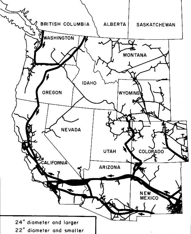
5.1. Natural gas pipelines—western states. Source: California Energy Commission (1981).
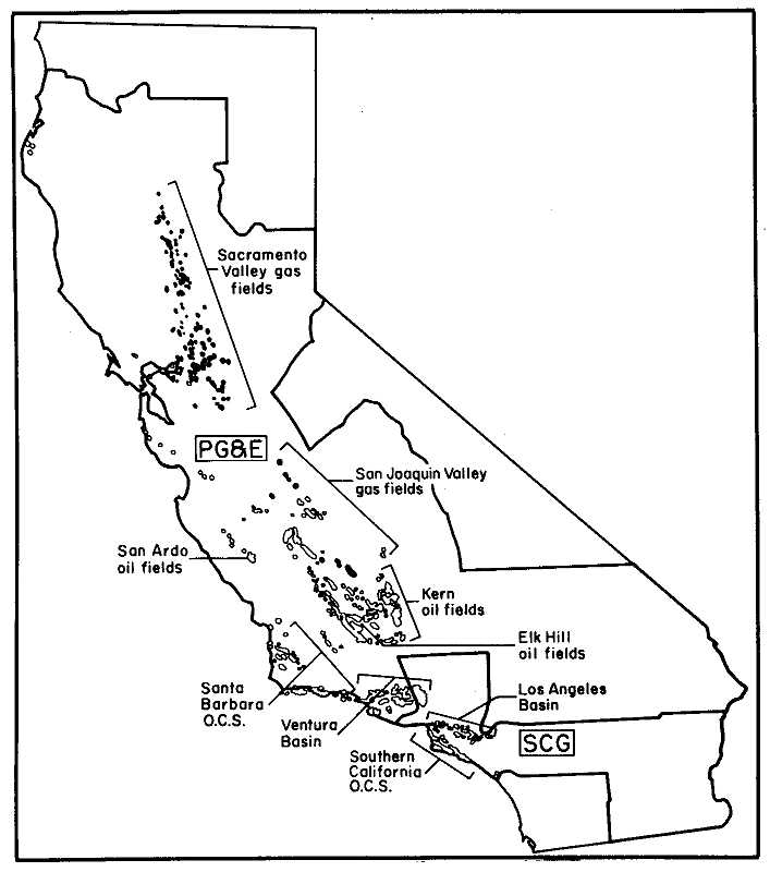
5.2. Gas utility service territories. Source: California Energy Commission (1981).
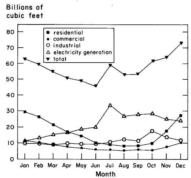
5.3. PG&E monthly gas deliveries profile, 1984.
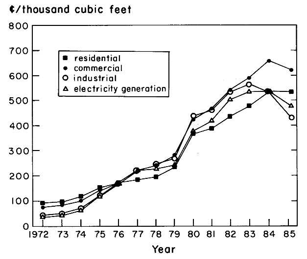
5.4. PG&E burner tip cost of natural gas by customer class.
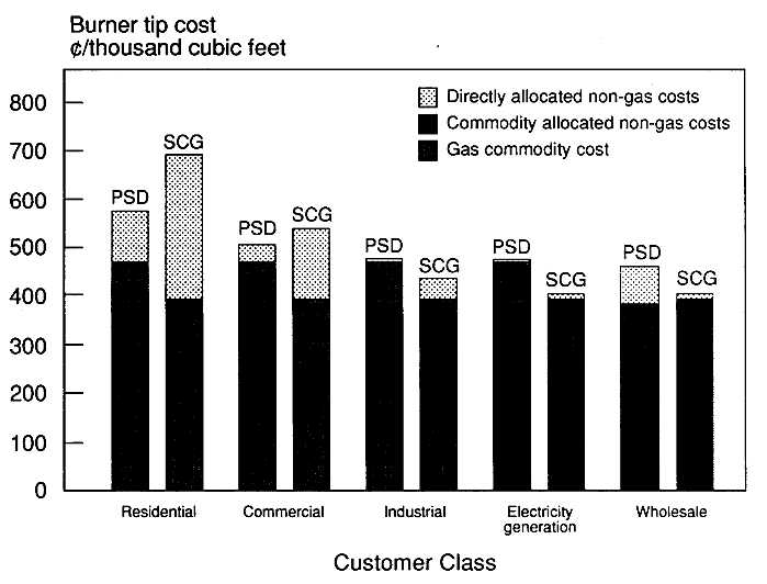
5.5. Imbedded cost of service estimates for SCG, 12 months beginning May 1, 1985.
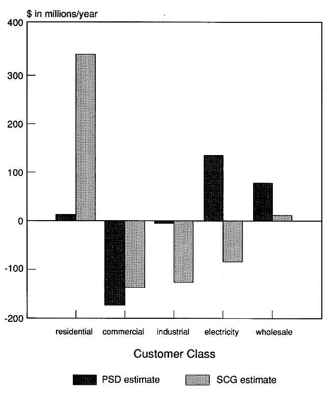
5.6. Estimates of total cross-subsidy for SCG. Positive value indicates recipient class.
SIX
Estimating Costs of Alternative Electric Power Sources for California
Walter J. Mead and Mike Denning
I. INTRODUCTION
The purpose of this chapter is to evaluate alternative electric power sources that will be available to the state of California in the next decade. The evaluation will be based on a conventional social benefit-cost analysis. We will draw on electricity supply-demand forecasts prepared by the California Energy Commission (CEC). These forecasts indicate that California "can meet all of its needs for electricity until the late 1900s" (California Energy Commission, 1987, p. 19). The alternative electric power sources we will evaluate will be imports from the Pacific Northwest, including British Columbia, imports from the Southwest, and new electric power sources that might be developed within California.
Forecasting energy demand and supply is not as simple as it was before the 1970s. At that time, prices for electric power fuel sources were relatively stable, resulting in relatively stable prices for electric power. Economic growth and population expansion produced steady growth in electric power demand at about 7% annually, enabling utilities to efficiently plan new power plant construction to meet demand expansion. The oil price revolution that began in the early 1970s brought these easily predictable conditions to an end when crude oil prices increased from about $3.25/barrel in the early 1970s to $39/barrel in February 1981. With similar price increases for substitute fuels, electric power prices increased and electricity consumption growth rates tumbled to about 2% by the early 1980s. Capital costs for new electric power generating plants also increased sharply in the mid and late 1970s. By July 1986, the price of U.S.-produced crude oil had fallen to $9.25/barrel, then nearly doubled to about $18/barrel by 1988. If oil and gas prices remain at or below present levels for several years and if no new generating
plants are built and qualifying facilities (OF) overpayments are eliminated, then electricity prices are likely to remain stable. In this event, growth rates for electric power consumption are likely to rise above 2% and return toward their pre-1970s levels, and California will need both new generating capacity and energy supplies well above those forecast by the CEC.
II. THE CALIFORNIA ENERGY COMMISSION SUPPLY-DEMAND FORECAST
The CEC and California public utilities face formidable problems as they attempt to estimate future electric power demand and supplies. Before the energy price revolution of the 1970s, with its induced demand shifts (conservation), supply-demand forecasting was a relatively simple matter of projecting past trends. In 1970 electric power was supplied from relatively static sources. In order of importance for the United States as a whole, they were coal, 49%; natural gas, 23%; hydro, 17%; oil, 10%; and nuclear, 1%. In California, oil and gas were the dominant energy sources, together accounting for 70% of the state's electric power generation. Coal combustion was not a source in California electric power generation. Nationally, coal prices were relatively stable. They were essentially constant from 1957 to 1967, when they started to increase at a 12.3% compound annual rate (nominal terms) through 1970.
U.S. residential electric power rates (nominal) were identical in 1940 and 1970, with only minor variations in the 30-year interval. Real prices (adjusted by the Consumer Price Index) declined by 64% from 1940 to 1970, a 3.3% compound annual decline rate. Given a 3.9% rate of increase in the real GNP over this period, one should expect a rapid growth rate in electricity consumption. Consistent with this expectation, electric power usage in the United States increased at an 8.6% rate over the three decades from 1040 to 1970.
In late 1972 oil prices started their upward spiral and, with a lag, produced major reductions in energy-use growth rates. Residual fuel oil prices started a tenfold increase in the last quarter of 1973. Electric power price increases followed with a lag of one or two years. These latter price increases continued into the mid-1980s, causing additional market-motivated conservation. Such dynamic changes suddenly made forecasts based on simple linear projections of past trends in electric power consumption virtually useless and required a new forecasting methodology in which sharp price increases and related changes in economic growth rates, as well as substitution of both old and new electric power generating technologies, would be taken into consideration. Finally, federal and state public policy became an important factor in determining electric power supply and demand.
In 1971 California public utilities projected electric power demand growth through 1980-1985 at a 7.38% annual rate, a reasonable projection given information available to the utilities in 1971. However, rapidly rising energy prices from 1972 through 1980 made this projection increasingly unrealistic. Average U.S. electric power prices (nominal) increased 3.4 times from 1973 to 1985 for a 10.8% compound annual rate. Real prices increased at a 3% annual rate. As should be expected, these rapid price increases caused electric power consumption growth rates to decline sharply. From 1975 through 1987, U.S. electric power consumption (with a two-year lag behind prices) increased at a modest 2.9% annual rate, and the growth rate declined progressively over this 12-year period. Reflecting this price-inspired conservation and (possibly) policy-enhanced trend, the CEC projected a declining electric power growth rate for California through the year 2005 in its December 1986 electricity demand study, as shown in Table 6.1.
However, the CEC electricity price forecast shows that the upward trend in electricity prices, which produced the observed decline in consumption, is expected to peak in 1988 and decline thereafter through the year 2005. Table 6.2 gives these projections, together with historical prices. Real prices increase at a 2.8% annual rate from 1977 through 1988 and then are forecast to decline at a 0.8% annual rate from 1988 through the year 2005.
Thus, although rising real electricity prices caused growth of electricity consumption to decline from about 7% annually before the 1970s to about 2% by the early 1980s, the CEC asserts that real energy prices will decline after 1988, but the rate of increase of energy consumption will continue to fall, as shown in Table 6.1. From an economic perspective, this CEC conclusion is difficult to accept. Instead, declining real prices should lead to increasing consumption growth rates toward, but not necessarily reaching, the 7% long-term growth rates realized before the energy crisis years. In fact, electric power consumption growth rates already show very sharp increases. Table 6.3 shows that twelve-month growth rates by month have increased to over 5% beginning in January, 1988. This matter is a serious one for California consumers of electric power. If electricity consumption growth rates are underestimated by the CEC and the actual growth rate turns out to be 3% between 1990 and 1997 instead of the 1.98% forecast by the CEC, then instead of meeting all electricity needs, we will suffer a shortage of about 13 billion kilowatthours. This shortage is the equivalent of about two nuclear plants of Diablo size (1100 MW operating at 75% capacity). Given the extremely long time period required to build new generating plants in California (construction of Diablo required 15.5 years), there will be no opportunity to construct efficient plants. Short-run solutions that are costly for ratepayers are likely to be sought as the only way out.
The CEC assessment of the need for new electric power supplies does not adequately consider the important economic forces that determine supply of and demand for electric power. The assessment gives little weight to electricity prices as primary determinants of electric power demand. Ignoring price implies supply and demand curves as shown in Figure 6.1.
The CEC 1985 electricity report "assessed" 1996 demand and supply, then subtracted one from the other, and arrived at shortage estimates for both generating capacity and energy in that year. Figure 6.2 shows the CEC forecast methodology in more detail: Starting with the 1983 actual load, the commission drew upon individual load growth forecasts provided by the state's utilities. The commission staff and commissioners reviewed and modified these forecasts to conform with their judgment.
Electric power supplies expected to be lost between 1983 and 1996 due to contract expiration (imports from the Pacific Northwest and the Southwest) and retirement of existing plants were subtracted from 1983 supplies and a difference identified as the basic need was calculated. This basic need appears to be independent of electricity prices.
In its 1981 biennial report, reaffirmed in 1983 and again in 1985 and 1986, the CEC determined that "after 1991 no more than one-third of the state's electricity generation (in GWh) should be fueled by oil or natural gas" (California Energy Commission, 1985a, p. 65). Accordingly, the 1996 supply assumptions show a reduction due to fuel displacement. The basis for the CEC policy of reducing oil-based electric power production is twofold: (1) a fear of another supply disruption and (2) expected crude oil price increases. In its 1985 energy plan, the CEC wrote, "Assuming no future oil supply disruptions, oil prices are expected to show average increases greater than inflation for the next 20 years" (California Energy Commission, 1985b, p. 20). This forecast was redefined in the CEC May 1986 energy demand report, which forecast that oil prices (real) would increase at a 3.1% compound annual rate for 1986 through 2005 (California Energy Commission, 1986a, p. B-8).
Regarding the supply disruption fear, the West Coast has what is commonly called the West Coast oil glut, a condition that started in 1977 with the flow of oil from Alaska's North Slope, constrained by a federal government ban on its export. The supply of oil available to West Coast refiners has recently averaged about 3 million barrels/day, while West Coast refinery crude runs are limited to about 2.2 million barrels/day. Thus there is an excess of about 0.8 million barrels/day that is disposed of by shipping or piping it through Panama and then into the Gulf of Mexico refining area. The last supply disruption experienced by the United States occurred in late 1973 as a result of the Arab-Israeli war. During a four-month period, the Arab members of OPEC imposed an
embargo on sales of crude oil to the United States, an action that reduced the world supply of oil by 6.6% (3.7 million barrels/day). At that time, neither the United States nor other large oil importing nations maintained stored reserves to compensate for an imposed disruption. However, the large importing nations now have some reserve capacity to offset the effects of an embargo. The U.S. Strategic Petroleum Reserve (SPR) alone has stored reserves amounting to 545 million barrels as of March 1988 (U.S. Department of Energy, 1988, p. 41). A supply disruption similar to the only one of consequence ever experienced by the U.S. would have no significant direct effect on West Coast crude oil supplies unless federal government regulations forced a reallocation of crude oil out of the West Coast.
Regarding the oil price issue, crude oil prices reached $39/barrel in February 1981, four years before the CEC 1985 energy plan was issued. As of January 1986, crude oil prices had fallen from their $39/barrel peak to about $21.46/barrel, a decline of 45%. From January 1986 through January 1988, instead of rising, crude oil prices (nominal) declined another 34% to $14.17/barrel (FOB cost of imports). Real prices for crude oil declined even more. The CEC policy regarding oil use in power generation was flawed not only in its incorrect price forecast, but also because of an essential distinction between baseload and peak load use of oil and gas energy sources. Capital costs of oil and gas plants for peak load power generation are relatively low, and oil or gas used in existing plants might be the least-cost source of meeting additional peak power demands. As a baseload source, oil and gas were certainly uneconomic at prices prevailing at the time of the 1985 policy statement. However, at less than $20/barrel for crude oil and approximately the same price for residual fuel oil, oil-fired electric power generation becomes worthy of consideration even for baseload power generation. This point will be discussed more thoroughly below.
The supply forecast was augmented by power supplies from likely additions. These additions consist of likely imports of power from the Pacific Northwest and the Southwest, plus projects that have been completed since 1983, are under construction, or are in various stages of CEC and/or California Public Utilities Commission (CPUC) approval.
The assessments outlined above leave a remaining 1996 energy need of 28,235 GWh of energy (6,349 MW of capacity). This gap may be filled by favored energy sources that have been reserved by the commission. Table 6.4 lists these reserved sources.
The commission makes clear that it will use its power to override the market and the judgment of utility companies to protect and advance its favored power sources. Its electricity report specifies that "only those resources for which the Commission wants to provide preference will have
an unfilled reserved need as of the adoption of this report. . . The Commission can clearly control approval of projects in its siting process that seeks to fill reserved need amounts, but must influence the decisions of other permitting authorities to encourage only those resources that provide the preferred mix that the Commission determines best meets state needs" (California Energy Commission, 1985a, pp. 76-77).
The projected 1996 deficit of 6,349 MW of capacity is approximately equal to three nuclear power plants of the Diablo Canyon size class.1 Whether this deficit will be filled by the sources preferred under the commission preference system is doubtful. First, 26% of that capacity is reserved for unspecified sources preferred by the commission. The remaining 74% would be forthcoming only if investors or decision makers conclude that the required investments would be relatively profitable. Most of the new in-state sources preferred by the CEC, including solar and wind generation, are uneconomic in the absence of government subsidies, as will be shown below and in Chapter 9. As the prices of oil and gas fall, alternative sources of electric power become less attractive. In the cases of both wind and solar power, the commission specifically notes that "the Commission's preference is for more than is estimated to develop" (California Energy Commission, 1985c, pp. 3-25). Even if the physical supply is forthcoming, the commission should have more concern for the costs that California consumers are required to pay.
As state and federal government subsidies are allowed to expire, the commission's preferred sources are not likely to fill the gap projected by the CEC for 1996 and beyond. In that event, plans should be made relatively soon to meet the projected electric power demand in the late 1990s. We now turn to an examination of the alternative electric power sources for California from both imports and development of new instate electric power sources.
III. POTENTIAL IMPORTS FROM THE PACIFIC NORTHWEST AND SOUTHWEST
Of the many possible future sources of electric power for California, importation of the large surplus of electric power from the Pacific Northwest and Southwest is potentially among the least costly. The cost of such imports depends on (1) intertie access policy and (2) Bonneville Power Administration (BPA) rates. The Northwest and its large network of hydroelectric generation sources has regularly had surplus electricity available for sale during times of heavy rainfall or runoff from snow-melt—typically during the spring and summer months. In the past few
years, however, a number of circumstances have led to a large surplus of electricity year round. That surplus is expected to last at least into the early 1990s and possibly until the end of the century.
In the Southwest anticipation of continued rapid population growth rates through the 1970s led to the construction of several new baseload coal-burning plants. In both the Pacific Northwest and the Southwest, growth in demand has been less than anticipated due to higher electricity prices and the 1980-1982 recession. Surplus generating capacity has consequently become available for California markets. The first five rows of Table 6.5 give the record of imports from each region.
The electric power imported from these regions is of two basic types—firm and nonfirm. Firm energy is electricity that is guaranteed to be delivered under contract. Nonfirm energy, on the other hand, is power that can be purchased only temporarily, according to its availability. Hydropower systems, such as those in the Pacific Northwest and the Hoover area in the Southwest, produce large amounts of nonfirm energy, because "critical water years" are used to plan for regional electricity loads, ensuring that even in a year with subnormal precipitation, utilities will be able to meet their local load requirements. Therefore, given normal precipitation levels, surplus nonfirm energy will exist year round, becoming particularly abundant in late spring and early summer as rivers swell due to mountain runoff. Available supply also depends on the relationship of storage volume to runoff volume. The Pacific Northwest stores only about 30% of its annual average runoff.
Firm capacity imports refer to purchases, exchanges, and entitlements to energy, from either utilities or specific generating units in other regions. Firm energy imports refer to purchases, under contract, of specified amounts (measured in kWh) of planned surplus energy from utilities in other regions. It should be pointed out that just because energy or capacity is labeled firm, it is not guaranteed to be delivered in all instances. The actual amount of power delivered under such contracts depends on the status of both the transmission system and the specific generating unit(s) from which the power is promised. Most interutility electricity sales are system sales. Because of the very small probability that a utility system will not be able to support a power contract, system sales are firm for planning purposes. On the other hand, power purchased from a qualifying facility2 (QF) is unit-specific and less reliable because it is not deliverable if the generating plant in question is unavailable. In some cases the importing utility is required to pay for contracted
power even if such power is not delivered. Therefore the prices bid for such energy and capacity reflect the estimated probabilities of transmission system and/or plant failure.
From a California perspective, firm energy is, when available, the most valuable of these two types for several reasons. If firm power can be purchased at prices below those of a utility's alternative power sources, the use of (formerly) expensive oil- and gas-fired peak load generating facilities may be avoided. In addition, long-term firm power is valuable to the extent that its availability allows California utilities to delay construction of costly new generating facilities. Nonfirm energy, although most plentiful (from the Pacific Northwest) during California's peak energy demand in the warm summer months, is least valuable because its delivery is not guaranteed, thus requiring backup sources of generating capacity to be maintained and run in years when nonfirm energy is unavailable.
Because firm power from the Pacific Northwest commands a higher price than nonfirm power and its availability can be planned, private utilities in the PNW prefer sales of firm power. Accordingly, Pacific Northwest utilities are attempting to firm up their generation system, through water storage and new generating techniques.
Pacific Northwest Imports
California utilities have regularly imported surplus power from the Northwest, but a majority of these transactions have been for nonfirm energy. Table 6.6 summarizes electricity imports from the Pacific Northwest for 1976-1985. Utilities in California and the Pacific Northwest are currently trying to make arrangements to capture more of the potential benefits from sales of surplus power by exploiting the current price difference and taking advantage of the differing seasonal demand patterns in each region. California utilities face their highest demand for electricity in the hot summer months, while the Northwest faces its peak demand in the winter when California demand is low. Consequently, both regions could reduce their required peaking capacity through exchange agreements whereby each imports peaking capacity during its peak season, repaying that electricity during the other's peak season.
The Northwest Power Planning Council (NWPPC) has suggested a number of strategies for maintaining the financial health of that region's electric power industry (Northwest Power Planning Council, 1985). These strategies include the development of a regional conservation plan, more efficient use of the hydropower system, reducing the load factor caused by aluminum industry cyclical demand volatility by increasing the interruptibility of this power, and the possible completion of two unfinished nuclear plants. Implementation of these measures
seems quite favorable for continued importation of power by California utilities.
Utilities in the Northwest and California are currently discussing long-term (15- to 20-year) contracts for firm electricity sales of approximately 1,500 MW of surplus capacity to California utilities (Bonneville Power Administration, 1983, p. 9). Based on existing and planned future construction, the NWPPC projects a surplus of 2,300 MW, which could last from 5 to 20 years, depending on load growth in the region. Rows 6 through 8 of Table 6.5 show California's projected imports from both regions through 2004. Actual levels will depend on transmission constraints, resource availability and prices, and the ability of California markets to absorb additional imports.
Another source of energy likely to be available for importation into California is British Columbia Hydro and Power Authority. B.C. Hydro has tremendous developed and potential electric power supplies and, with actual Canadian demand less than forecast, is anxious to increase revenues by exporting surplus electric power. In addition, the provincial government is currently proposing that B.C. Hydro build projects to generate power dedicated solely for long-term firm export to the western United States. Another advantage is that B.C. Hydro draws much of the water for its hydroelectric generating facilities from areas unconnected with the sources of Pacific Northwest water. Consequently, a poor water year in the Pacific Northwest may not affect exportable energy from B.C. Hydro. Also, B.C. Hydro's capacity to store water is much greater than that of Pacific Northwest utilities, creating attractive possibilities for firm sales with increased supplies in the late autumn and early winter when the Pacific Northwest normally has little or no surplus. Based on its 1983 load forecast, B.C. Hydro is expecting energy surpluses of about 10,000 GWh currently, declining to approximately 800 GWh in 1996-1997 (see Table 6.7). Given average water conditions, these surpluses may be even larger by as much as 4,000-4,500 GWh/year.
The major obstacle B.C. Hydro faces in exporting power to California is a lack of transmission capacity. Existing capacity to the intertie system at the U.S./Canada border is 2,000 MW, which could be increased 300-400 MW at a nominal cost. Due to BPA's current intertie access policy, B.C. Hydro has last priority on use of the intertie. One way in which B.C. Hydro can circumvent this constraint is by selling water to BPA, who then generates power and sells it over the intertie. BPA can also sell power to the Pacific Northwest if the demand exists, allowing Pacific Northwest utilities the option of reselling this displaced power in California markets. BPA is currently blocking these purchases. If B.C. Hydro is afforded greater use of the intertie, it would consider building a large hydro project (Peace Site C) earlier than its proposed 2002 startup
date. This would increase exportable capacity by 900 MW (4,500 GWh of energy) (British Columbia Hydro, 1985). Currently, utilities from California, the Pacific Northwest, and British Columbia are jointly studying the feasibility of the Peace Site C dam. If the assessment is favorable, it appears that BPA's long-term intertie access policy will allocate a much larger portion of intertie capacity to B.C. Hydro. This would make possible the purchase of large amounts of valuable long-term firm energy from B.C. Hydro by the early 1990s.
Any electricity transferred between these regions must travel over the Pacific Northwest-Pacific Southwest Intertie. This network consists of one dc and two ac transmission lines that run from northern Oregon to southern California. The total carrying capacity at present is 5,790 MW. Plans to further upgrade the system by building an additional ac line are currently under the process of review for certificate of convenience and necessity. This line would raise the carrying capacity by approximately 1,600 MW at a cost of $450 million in 1968 dollars (l.4¢/kWh) (California Energy Commission, 1986b, pp. 5-19 — 5-20).
In the past few years, the price of imports from Pacific Northwest utilities has risen from 0.5¢ to 2.3¢/kWh, due mainly to BPA's intertie access policy, which has reduced competition and eliminated the low spill rates formerly applied during very high water levels.3 Because future rates have not been firmly established, there is some speculation as to whether California will continue to import enough power from the Pacific Northwest to justify construction of this additional line. Barring additional long-term quantity and price commitments for both firm and nonfirm energy, it appears unlikely that the expenditure for any transmission capacity upgrades will be economically justifiable. The intertie expansion issue appears to be a "Catch 22" situation—without assurance of available transmission capacity, buyers and sellers are reluctant to enter into sales contracts, but without transmission contracts, funds for expansion of the intertie are unlikely to be available.
In addition to its existing capacity, the Pacific Northwest has two nuclear plants that were slated for completion in the mid-1980s but that have been delayed due to existing surplus capacity in the region. The NWPPC estimates that the present value of net benefits of finishing these projects is $630 million (Nucleonics Week, 1986). Construction on these plants, referred to as Washington Public Power Supply System (WPPSS) numbers 1 and 3, is scheduled to be restarted and completed when the need for additional capacity in the Pacific Northwest becomes apparent. These plants represent an additional 1,600 MW of generating capacity that could be available in the not-too-distant future. To date, $4.4 billion has been spent on these two projects, and the estimated in-
cremental cost to complete both plants is $2.76 billion (1984 estimate). The preservation costs are $52 million per year.4 Given these figures, had construction resumed on plants 1 and 3 in 1988, the levelized cost (completion, operating, and finance costs) would have been around 3.7¢/kWh (Bonneville Power Administration, 1984). If construction were to resume at a future date, the levelized cost would be higher because of additional preservation and maintenance expenditures.
Although authorities in the Pacific Northwest are striving to bring about the completion of these plants, they face a number of problems in achieving that goal. BPA, the owner of these plants, does not plan to complete them as a source of exportable energy but will only consider completion if and when the Pacific Northwest region's load growth makes them economic and financing becomes possible.5 Based on current supply-demand projections, the earliest that either plant could be on-line is 1992, with the most probable startup date being 1999.
California utilities might consider purchasing one of these plants for some share of the sunk costs and then completing and operating it with power dedicated to California. Because these plants can be completed by BPA and brought into use if regional loads grow faster than expected, they are valuable as options and probably would not be sold until they appear to be uneconomic for meeting future loads in the Northwest. Whether such a transaction takes place is likely to be decided on political bases, regardless of the economic costs and benefits.
In the event that additional electric power supplies from the Pacific Northwest or British Columbia become available to California, further expansion of the intertie could become necessary. In addition to the aforementioned construction of an ac line from John Day Dam in northern Oregon, to Tesla, California, another proposed addition is a large dc line from Celilo, Oregon, to either Mead, Nevada, or Phoenix, Arizona. This project would add 2,000 MW of capacity to the system at a cost of approximately $1 billion (1985 dollars) (California Energy Commission, 1980). The transmission capital cost would then be 0.6¢/kWh (assuming a 35-year lifetime and a 5% real interest rate, and a capacity factor on the line of 60%). The cost of these transmission upgrades is relevant to the decision of whether developing new B.C. Hydro supplies or completing the WPPSS plants would be most economic for California utilities, because the total incremental cost of that energy delivered to California is the incremental production cost plus the incremental transmission cost.
The groups likely to be most affected by the outcomes of these negotiations are the ratepayers in the two regions. Pacific Northwest utilities
can maintain lower rates by taking advantage of seasonal diversity through power exchanges and supplementing their revenues with surplus power sales. By importing power at a price lower than other alternatives and covering the summer peak demand with power exchanges from the Pacific Northwest, California utilities will also be able to maintain lower prices and further delay capital expenditure for new capacity. In addition, if either one or both of the WPPSS plants were found to be uneconomic in the Northwest and were sold to California utilities, rates in the Pacific Northwest would decrease because payment of some portion of the sunk costs of the project would be required to gain ownership. If the plants (1 and 3) are not used or sold, Pacific Northwest rate-payers or financing interests stand to lose all of the costs accumulated up to that point.6 Benefits to California ratepayers would be in the form of reduced electricity rates if the incremental costs of the power generated at these plants and delivered to California is less than alternative new baseload sources.
There are problems related to importing additional power from the Pacific Northwest. BPA is obligated to serve the utilities in its area before it can sell to others outside the region. A BPA agreement to supply firm power outside the region requires (by the Pacific Northwest Preference Act of 1964) a clause allowing the agreement to be cancelled with 60 days notice. The option to cancel reduces the value of this power, a point that California utilities must carefully consider before entering into contracts with BPA. Recently, BPA devised firm displacement rates to eliminate this problem. This innovation allows BPA to sell firm power to other Pacific Northwest utilities at a set price, enabling those utilities to individually sell short-run firm power and negotiate a higher price. This arrangement, along with the current intertie access policy, improves prospects for importing firm power from the Pacific Northwest. This development still fails to meet a California need for long-run firm baseload power to meet requirements around the turn of the century and later.
There are two operating constraints that also affect the ability of the California system to accept Northwest imports (California Energy Commission, 1984). First, utilities in California rely on gas- and oil-fired steam boilers for peak load requirements, a use for which these technologies were not designed. Many of these units cannot be taken from a cold shutdown to full output in a short period of time; they must be operated at some minimum level before being available to meet peak loads. This minimum generation requirement reduces the amount of gas and oil generation that can be displaced by imports, especially of nonfirm power, and thereby decreases the value of this power. Second, the addi-
tion of several baseload nuclear plants in California and lower oil and natural gas prices have greatly decreased the variable cost of baseload generation. This has led to a situation in which even nonfirm deliveries from the Northwest (at about 2¢/kWh in 1988) have become more expensive than the variable cost of baseload sources in California. The value of Northwest energy is then dependent on the types of generating capacity it replaces and is further diminished when northern California has good rainfall, which increases the amount of low-cost hydroelectric power available within the state.
Currently, California's demand for Northwest imports to displace existing baseload generation is very small, whereas the demand for power to displace the more expensive oil and gas generation needed for peaking requirements is great. At previous oil and natural gas prices, firm energy could be purchased for a price one-fourth the cost of operating these peaking generators. This leads to further discussion of the benefits derived from importation of electricity (largely firm energy and capacity) from the Southwest.
Southwest Imports
Southern California utilities have been importing a large portion of their baseload resources from the Southwest for a number of years. These resources have come from jointly owned coal plants located in the Southwest, purchases of firm surplus capacity and energy from Southwest utilities, and firm purchases from federal hydroelectric facilities on the Colorado River. Lower-than-expected electricity demand in this region, due to a depressed mining industry, energy conservation, and the recent recession, has led to surplus generating capacity and nonfirm energy, especially in the Rocky Mountain states. California utilities are counting very heavily on this region as a source of continued future imports for at least the next 20 years, as is indicated by the projections listed in Table 6.5. The surpluses in the Southwest are a product of the large fluctuations in daily and seasonal loads, as well as the large base-load component of Southwest generating capacity.
The Arizona-New Mexico-West Texas area and parts of Colorado, like California, are summer peaking, whereas the Rocky Mountain states are winter peaking. More than 60% of the region's generating capacity is coal-fired, with 25% oil- and gas-fired generation. The total capacity is around 30,000 MW and the region's reserve margin in 1985 exceeded 35% (California Energy Commission, 1985d, p. 42). California utilities currently own shares in five Southwest area coal-burning plants and have plans to further increase their ownership in out-of-state coal plants in Nevada, Utah, and New Mexico, as well as nuclear plants in Arizona. These additions would more than double the currently existing
California-held capacity from 2,445 MW to 5,372 MW. California utilities are now buying firm capacity and energy from Southwest utilities, and additional firm contracts are being offered.
The fully allocated total costs of new Southwest baseload construction, including transmission costs, is between 5¢ and 7¢kWh (1985 dollars) (California Energy Commission, 1984). The variable operating costs of Southwest coal plants range from 0.4¢ to 1.6<0162>/kWh. Thus, if excess capacity exists, the relevant economic cost for export sales is quite low. The cost of Southwest nonfirm energy has been in the range of 1.1¢ to 4¢/kWh since 1980. Nonfirm energy costs in 1987 averaged 2.1¢/kWh. Low production costs in the Southwest, in the range of 1-1.4¢/kWh, could allow for further reductions in nonfirm prices, making them very competitive with Northwest prices.
The existing transmission network is adequate for firm energy transfers, but there have been problems in transferring the current levels of nonfirm energy. Recent studies recommend that simultaneous California import capacity (between the Southwest and Northwest) be reduced to correct problems encountered in transfers between Arizona and California. These problems, including loopflow,7 are due to operation of the Pacific Northwest intertie at high levels and have in the past necessitated the reduction of southwest imports into California. Operation of the Southwest powerlink, a line between Arizona and southern California that was completed in 1984, and the IPP lines, which were completed in 1987, provides a near term solution to this problem. In the longer term, major upgrades of the transmission system may become necessary (California Energy Commission, 1984).
A major transmission project, Palo Verde-Devers #2, has been issued a certificate of public convenience and necessity. However, approval was granted on the condition that the CPUC would have to reconsider the need for the line if the proposed merger between Southern California Edison (SCE) and San Diego Gas and Electric were consummated. According to testimony submitted by Joe D. Pace on behalf of SCE in the FERC hearings on the merger, this line is currently scheduled to become available for commercial operation in June, 1993 (Federal Energy Regulatory Commission, 1989).
The addition of this capacity would raise total transmission capacity from the southwest of California from 5,700 to 6,900 MW. The Palo Verde-Devers line could relieve transmission problems that have, in the past, precluded the importation of considerable surplus energy from Colorado, New Mexico, and Utah. Recent forecasts show that the existing and planned transmission facilities should be able to accommodate the projected levels of nonfirm energy imports from the Southwest.
Summary
Electric energy imports are expected to increase (see Table 6.5) in the short term as transmission capacity between California and both the Pacific Northwest and the Southwest increases, new generation facilities come into service, and load management and hydro system enhancement programs continue to be implemented. In the long term, however, importable energy is expected to diminish as demands in the source areas increase, new generating capacity is brought in at a slower pace in the Southwest, and normal precipitation patterns return to the Northwest. As economic prosperity and population growth continue over time, the demand for electricity in California will also increase. The combination of diminishing supply and increasing demand for electric power imports by California utilities will lead to a declining proportion of California's electricity requirements being filled by imported energy. This is not necessarily detrimental for California utilities as there is strategic value associated with in-state gas, oil, and (in the future) possible coal and nuclear generation. The natural gas and coal plants have value as a source of backup energy in the case of performance difficulties encountered with existing nuclear plants, intermittent wind or solar plants, or nonfirm imports. Thus the existence of these plants reduces the probability of California utilities having to make expensive emergency purchases. Also, at present they contribute some firm capacity value to in-state hydro and nonfirm hydro purchases from other regions. Thus there is justification in assigning some added value to in-state generation when comparing it with the cost of out-of-state purchases. (California Energy Commission, 1985a, p. 134).
The level of future imports from the Pacific Northwest is somewhat more uncertain than that from the Southwest, mainly because of the uncertainty associated with the price and availability of that power. BPA, through its intertie access policy, has reduced competition in the supply of Pacific Northwest power, greatly reducing the benefits California utilities receive from such purchases. Rates for nonfirm surplus have increased eightfold since 1979 (California Energy Commission, 1985a, p. 137), and efforts to negotiate long-term rate agreements have been fruitless. Rather than face the risks posed by relying on energy the price of which may be subject to complete control by BPA, California utilities are encouraged to develop cost-effective alternative Southwest or indigenous firm power resources, while leaving open the option to import power if agreements are reached in the future.
The current capacity of the transmission facilities between California and the Pacific Northwest is insufficient to accommodate the potential power transactions between regions, especially in the spring and summer months. One effect of this is that B.C. Hydro, which receives last priority on intertie use, yet which has large exportable supplies, is
severely limited in its ability to sell to California utilities. In addition, most California utilities are participating in the California/Oregon transmission project, despite their inability to negotiate long-term agreements with Pacific Northwest utilities.
The emergence of B.C. Hydro as an important source of low-cost firm energy imports seems almost certain in the near future. As the Pacific Northwest regional surplus declines in coming years, B.C. Hydro, with its large capacity, tremendous resources, and desire to increase its revenues through energy exports, may have the opportunity to greatly increase its sales to California. Although B.C. Hydro controls none of the intertie system, as excess transmission capacity becomes available, the utility will be able to gain greater access to the network, wheeling its power through intertie owners.
Because surplus energy currently exists in the Southwest, as well as adequate transmission capacity to further expand import levels, California utilities are anticipating substantial electric power imports from that region. Also, with the planned additions to the transmission network in the region, import levels will increase even further. Southwest utilities are likely to continue to build mainly coal-fired baseload plants as long as coal prices remain low compared with other fuels. They may also continue to build in excess of their own requirements, depending on the price of surplus energy, the potential for long-term contracts for firm energy, the accuracy of their demand forecasts, and the relative costs of other generation techniques.
Because considerable exportable surpluses of energy exist in both regions, it appears that California utilities can assume that they will be able to make the desired purchases from both regions. One reason for this is that California is the main, if not only, customer for this energy. Either region would therefore be foolish to set high prices that lead California to develop lower-cost alternative sources. If Pacific Northwest power becomes too expensive for continued importation, California utilities will likely be able to rely on B.C. Hydro for increasing amounts of power (if BPA grants intertie access). Therefore, although long-term agreements have not been made with Pacific Northwest utilities, surplus power prices should remain in the range in which California utilities will continue to benefit from such purchases.
IV. ALTERNATIVE NEW CALIFORNIA IN-STATE ELECTRIC POWER SOURCES
In addition to imports of electric power from the Pacific Northwest and the Southwest, California may develop new sources of electricity from in-state investments. These new sources begin with conservation, which
might reduce energy use and therefore reduce the need for new energy sources. More generally, energy may be produced from increased investment in conventional sources of electric power, including coal, natural gas, oil, and nuclear electric power generation. Renewable resources including hydro, solar, and wind energy may be converted into electric power. There is some hope that in the more distant future, nuclear fusion might be a source of nearly unlimited electric power. Finally, miscellaneous sources, including biomass incineration and electric power storage, which expand peak load supply, may offer relatively small increments of electric power. We will consider all of the sources listed except the small increment sources. Geothermal is a major source of electric power in California providing 18% of Pacific Gas and Electric Company's 1986 generation. It is also a potentially large source for future development, although the best sources have already been developed.
Before we examine the cost of some of the alternative energy sources listed above, a methodology for evaluation should be specified. Economists have developed an evaluation system known as benefit/cost analysis for evaluating the relative merits of alternative systems for accomplishing some objective. The subject of analysis in the present case is production of a homogeneous good—electricity. Its benefit is its social value per kilowatthour, multiplied by the number of kilowatthours consumed. Its cost is the value of resources used up in its production process.
A distinction must be made between private investment analysis and social benefit/cost analysis. The former evaluates a proposed investment by identifying the costs paid by the decision-making firm (or individual) and the revenues expected to be received by the firm. Social benefit/cost analysis goes beyond private analysis to identify any costs borne by society at large but not by the decision maker, as well as any benefits that spill over to society at large but are not collected by the decision maker. These spillover costs or benefits are also known as external costs or benefits.
Private decision making based on analysis of private costs and private revenues yields the same results as social benefit/cost analysis in most cases. They differ only when (1) externalities exist, (2) monopoly power distorts prices, or (3) government(s) interfere in markets and distort resource or product prices.8
An example of external cost is air pollution, which is imposed on society at large or on one's neighbors but is not paid for by the decision
maker. Such external costs may be internalized without government intervention when legal action is instituted against a polluter or when a bargain is struck between the parties. In this event, the externality no longer exists. Similarly, an externality exists when a benefit accrues to society at large and cannot be collected by the decision maker who made it possible. An example is a discovery of a nonpatentable basic scientific fact, such as the nature of nuclear fusion.
Most ordinary business decisions do not create significant externalities. Therefore private decision making is in harmony with the general welfare of the society in question. Even when some external costs or benefits exist, they may be minor relative to the costs of correcting them and are therefore best ignored. When externalities are large, then some government intervention might be desirable only if such intervention is likely to improve on resource allocation by internalizing such externalities.
In the analysis to follow, we will examine the benefits and costs of alternative energy sources available to California. Only in the cases of nuclear and conventional coal-fired electric power generation do the external costs appear to be potentially significant. Therefore they will be evaluated in detail.
Major external costs would occur in the event of a meltdown in a nuclear plant or other accident in which a significant amount of radiation is released into the atmosphere. Coal-fired plants may impose externalities because large segments of the population downwind from a coal-fired power plant may suffer from respiratory problems. Both acid rain and the greenhouse effect are potential external costs of coal combustion in electric power generation. Solar and wind conversion systems may offer external benefits. Such potential benefits would be in the form of technological spillovers—declining costs over time as technology advances. Past large federal and state subsidies have paid or possibly overpaid for these potential external benefits.
The reader must be cautioned that the cost estimates shown below are from a variety of sources. Analytic methods are not likely to be uniform. Consequently, cost estimates should be taken as rough approximations of actual costs.
Conservation
People outside the circle of professional economists frequently use the word conservation as if it were a source of energy. From an economic theory perspective, there are two reasons to expect reduced consumption corresponding with higher crude oil prices. First, Figure 6.3 shows that if prices increase from P 1 to P 2 , the quantity demanded in the short
run will decline from w to x. In response, oil consumers shift to the most attractive substitutes. However, this substitution process requires a delay as oil consumers use the available information to determine which substitutes are optimal for their particular needs. Thus in the long run consumers and industrial users reduce oil consumption in favor of coal, natural gas, or other energy forms economically substitutable for oil. The longer the period, the greater will be the reduction in demand for the higher-priced oil.
Second, the demand curve may shift as consumers reallocate their scarce income and consume less higher-priced energy in total, including oil. Again, time is required for this income adjustment process. Thus in the short run the demand for crude oil will be highly inelastic (insensitive to oil price changes) but will become more elastic with the passage of time, as illustrated in Figure 6.3.
Some advocates of conservation frequently have in mind a set of government policies inconsistent with the economic meaning of conservation. These policies include new regulations that mandate less energy use, even though consumers would use other resources in lieu of the one constrained by regulation. Illustrations of this policy include mandated home insulation retrofit in order to save energy, without considering the other resources used in the retrofitting process such as the insulation material, labor, nails, etc. Another kind of conservation policy would add taxes to existing prices of specific energy forms. Examples include a gasoline tax and an import tariff on crude oil. Finally, a more benign form of market intervention simply mandates that manufacturers provide more product information to consumers about energy usage, as in the cases of refrigerator and air conditioner energy consumption. Such policies are inconsistent with the economic definition of conservation in all cases where the present value of the benefits (energy saved) is less than the present value of the substitute resources used, together with regulatory costs.
From an economic perspective, the word conservation has a precise but somewhat difficult definition. Conservation of resources takes place when the present value of the consumption of all resources is maximized. In practice, this means that private and governmental users of resources consider the costs and the benefits (or revenues) that are incurred as they make investment and consumption decisions regarding the use of resources and make those investments only when the present value of the benefits exceeds costs by an amount that yields a competitive rate of return. The great merit of this definition is that it leads to conservation of all resources, not just the one that is the target of a specific regulation or other government policy. This economic definition
serves the general interest of society if external costs and benefits are negligible or nonexistent and there are no market distortions due to monopoly or to government intervention.
Advanced Coal Combustion and Coal-Derived Synthetics
Coal is an alternative to crude oil in several applications. Recoverable reserves of coal in the United States and worldwide are extremely large; world coal reserves are 493 billion short tons (2,219 billion barrels of oil equivalent), of which 34% are in the U.S. The heat content represented by these coal reserves is 4.7 times the heat content of the world's estimated recoverable crude oil reserves.
Coal can be liquefied into a crude oil substitute; it can be gasified into a substitute for natural gas that, in turn, is a substitute for crude oil; it can be gasified and burned directly in a gasification combined-cycle electric power plant, or it can be either indirectly or directly converted into gasoline. It can also be burned in conventional electric power generating plants as a substitute for nuclear energy, residual fuel oil, or natural gas.9 We consider coal liquefaction, gasification, gasification-combined cycle (GCC), and conversion into gasoline because if these processes are economically viable, their large-scale development would affect oil or natural gas demand and prices and therefore the use of these energy sources for electric power generation.
Fluidized-Bed Combustion. In addition to the conventional method of coal combustion for electric power generation, a new process in the technical development stage and not fully proven commercially is fluidized-bed combustion (FBC), which encompasses both atmospheric (AFBC) and pressurized (PFBC) technologies. Bubbling bed and circulating bed are two types of pressurized FBC. The advantages of FBC relative to conventional coal combustion are short construction time, low emissions of both sulfur and nitrogen oxides, fuel flexibility, compatibility for plant retrofits, easier handling of residual products, potential economic feasibility for small-scale operations, and possibly more competitive capital and operating costs in the future.
Offsetting these advantages to some unknown degree, however, is the unproven reliability of large-scale systems and hence the actual costs of the power produced. Furthermore, turbulence in the bubbling bed, which keeps coal particles suspended inside the combustor by air jets, erodes the metal boiler tubes that run through the beds. A joint federal government and privately funded research project was announced in
early 1988 to solve this problem (Oil Gas Journal, 1988, p. 16). American Electric Power Company will retrofit its idled Tidd coal-fired plant in Ohio for a FBC process to study this issue. It will become a 70-MW capacity pilot plant and if successful, would be transformed into a 320-MW commercial plant, demonstrating retrofit feasibility. Based on information gathered from several small-scale testing facilities, there is some evidence that FBC may make coal-fired power generation an environmentally and economically attractive source of electric power in coming years.
The AFBC electric power generating process burns coal with limestone in an atmospheric pressure fluidized bed suspended by air blown in from below the combustion chamber. The calcium in the limestone captures most of the sulfur released from the coal during combustion. Particulates are captured in a series of cyclones followed by an electrostatic precipitator (Electric Power Research Institute, 1986, p. B-50). Using a fluid boiler design based on the bubbling bed concept, the Electric Power Research Institute (EPRI) has estimated the cost of a 500-MW (net) plant having a capital cost of $1,274/kW of capacity. Using a 7% real interest rate and a 40-year life, the cost of electric power from an AFBC plant is estimated to be 4.41¢/kWh in 1987 cents. Components of this estimate are illustrated in Figure 6.4 (see the bar labeled e ). This figure compares the costs of alternative electric generation technologies discussed below. Included in the comparison are cost estimates for new technologies (such as AFBC) and actual costs for some technologies presently deployed on a commercial scale.
PFBC is another new technology currently under development that uses coal to produce electric power in a more environmentally acceptable manner. In this process, crushed coal is burned with dolomite in a pressurized fluidized bed suspended by air blown in from below the combustion chamber. Pressure in the combustion chamber is maintained at 6-10 times atmospheric pressure. Sulfur particulates are removed by a filter after the hot gases leave the combustor and before the gases are used to drive a gas turbine/electric generator (Electric Power Research Institute, 1986, p. B-52). Based on EPRI data, the cost of power generated by the PFBC process is estimated to be 4.78¢/kWh in 1985 dollars, or 5.05¢ when inflated to 1987 prices (see the bar labeled f in Figure 6.4).
Both AFBC and PFBC plants are in the developmental stages with some retrofits already in use. With their estimated costs being only marginally above conventional coal combustion processes, they offer a promising method of utilizing the large U.S. coal reserves without the troublesome environmental and health consequences of conventional coal combustion.
Neither the availability of large-scale reserves nor the technical feasibility of liquefaction, gasification, or FBC are sufficient evidence that coal is an economic substitute for crude oil. Economic feasibility depends on relative social costs and benefits. The costs shown here are private costs. If the externalities of FBC are not significant (as we believe), then the private cost estimates are reasonable approximations of social costs, and FBC appears to be a promising alternative future source for California electric power generation.
Coal Gasification-Combined Cycle (GCC). Coal may be gasified and then directly burned in a gas-fired electric power generating plant. Operating experience is available from a semicommercial integrated coal gasification-combined-cycle plant at Daggett, California. This plant, known as Cool Water, has been operating since its startup on June 1, 1984. Its net capacity is 103 MW, and it operated at 70.5% of capacity in 1987. Its actual capital cost was $279 million. However, its operator, Southern California Edison, estimates that a similar new plant could be built for approximately $250 million. Using this capital cost, a 7% real interest rate, a 30-year life, and a 65% capacity factor yields an 8.21¢/ kWh cost for electric power production, broken down as shown as bar g in Figure 6.4. In converting 1,000 tons of coal per day into relatively clean-burning gas, air emissions from this plant average about 10-20% of the allowable federal levels for nitrogen oxide, sulfur dioxide, and particulate emissions. At a cost of 8.21¢/kWh, new construction of a GCC plant is not economic relative to other baseload options. However, one might expect further technological improvements in this process. Costs must be reduced by another 50% from these estimates before the GCC alternative becomes attractive.
EPRI has estimated cost data for a plant nearly five times as large as the semicommercial Cool Water plant. Based on a 500-MW net plant capacity, a 30-year life, 7% real interest, coal at $1.52/million Btu, and a heat rate of 9,775 Btu/kWh, the EPRI data indicate a cost of 4.60¢/kWh. Expressed in 1987 prices, this cost becomes 4.85¢/kWh. Thus, a larger plant would appear to incur costs that become attractive when consideration is given to the clean-burning character of GCC compared to conventional coal. Components of this estimate are shown as bar h in Figure 6.4.
Coal Liquefaction. Coal reserves may also be converted to synthetic oil. The proposed Breckenridge coal liquefaction plant, designed to produce 4.2 million barrels of synthetic oil per year, involved a conversion
cost of $96/barrel of oil output in 1987 dollars.10 This is more than five times the current value of imported oil ($14-$20/barrel). Accordingly, given present technology, coal liquefaction does not appear to be a viable substitute for crude oil in the foreseeable future.
Coal Gasification. Coal gasification is similarly uneconomic. The Great Plains coal gasification plant, partially financed by the U.S. government Synthetic Fuels Corporation, started production in July 1984 but is currently in bankruptcy following withdrawal of the federal subsidy. The cost of converting coal into high-Btu (970 Btu/cubic foot) gas is $8.59/thousand cubic feet in 1987 dollars.11 This is nearly five times the current market value of natural gas ($1.74 wellhead price, March 1988). Thus coal gasification also appears to be uneconomic for the foreseeable future.
When the Great Plains plant emerges from bankruptcy, the capital cost of $4.08/thousand cubic feet is likely to be eliminated. The most recent operating data for this plant show that operating costs have been reduced to $4.13/thousand cubic feet (U.S. General Accounting Office, 1986, p. 23). The free-market price of natural gas has fallen more than coal prices and well below this operating cost, indicating that the plant is still not economically viable even when omitting the capital cost. In the unlikely event that the value of natural gas exceeds the variable cost of operating and maintaining the plant at the time it emerges from bankruptcy, continued operation of this existing plant would be expected. However, construction of additional coal gasification plants would involve new capital costs and hence such additional coal gasification facilities clearly would not be economically beneficial in the foreseeable future.
Coal to Gasoline. A technology also exists for converting coal directly into gasoline as a substitute for crude oil. With substantial government subsidies, gasoline is produced in South Africa from that nation's large coal reserves. Hitler's Germany produced both oil and gasoline from German coal in World War II. In both cases, government subsidies can be and were justified on the grounds of supply security.
More recently, West Germany constructed a pilot plant to test the production of gasoline from coal using the Mobil M process in a plant near Bonn, Germany. The results established the technical feasibility but economic infeasibility of this coal substitution for crude oil in gasoline production.12 The Bechtel Corporation had earlier estimated that a commercial plant to produce gasoline using the Mobil M process would have a capital cost of $6 billion and that, using a 7% real interest rate, a 30-year life, and a favorable 90% capacity factor, the cost would be $0.8l/gallon (1981 U.S. dollars). This capital cost alone is now approximately 1.6 times the tax-free market value of gasoline. In addition, the cost of coal and operation and maintenance must be borne by the product. In the absence of data on these costs, we roughly estimate them at $0.80/gallon, making the total cost of coal conversion to gasoline about $1.60/gallon in 1981 dollars, or $2.20/gallon in 1087 dollars. These results indicate that this process is uneconomic.
Natural Gas to Gasoline
New Zealand's Synthetic Fuels Corp., Ltd., entered into an agreement with Mobil Oil Corporation in 1980 to build the world's first natural gas-to-methanol-to-gasoline plant using a catalyst developed by Mobil Oil. The lead contractor was Bechtel Pacific Corp. The source of natural gas is the Maui field off the New Zealand coast. This plant has a design capacity of 14,500 barrels/day of gasoline. The capital cost is estimated at U.S. $1.475 billion (Oil and Gas Journal, 1985). The capital cost alone, assuming a 30-year life, a 7% real interest rate, and an optimistic 90% capacity factor, amounts to $0.60/gallon of gasoline (U.S. dollars). As of May 6, 1988, the wholesale spot market price of regular gasoline (excluding tax) in Rotterdam was $0.51/gallon. Thus at zero operating cost, the capital cost alone of gasoline to New Zealand will be more than its market value. Although operating costs are unknown, they are likely to be at about one-half of the capital cost estimated above ($0.25/gallon). The cost of natural gas, valued as low as $2/thousand cubic feet (U.S. dollars), would be $0.43/gallon of gasoline. Therefore natural gas conversion to gasoline costs about U.S. $1.20/gallon, 2.3 times the value of gasoline, in 1984 U.S. dollars. Inflated to 1987 prices, this cost becomes $1.30/gallon. Thus, natural gas conversion to gasoline as a substitute for crude oil is clearly uneconomic.
Oil Shale
Oil shale resources, like coal, are extremely large. Unlike coal, however, oil from shale is not economic under present technologies, costs, and
prices. World oil shale resources are estimated at 88 trillion tons (World Energy Conference, 1983, p. 51). If 10% of this resource ultimately became recoverable, it would amount to nearly 400 billion barrels of oil.
But the economic reality of producing oil from shale is harsh. Current estimates indicate a range from $45 to $60/barrel production costs. Furthermore, the history of oil shale suggests that its production cost increases in tandem with expected revenue. Consequently, oil from shale is not a viable substitute for crude oil under present costs and prices.
Tar Sands
Tar sands and heavy oil resources are very large and are being produced in Alberta, Canada, and California. In addition, heavy oil resources in the Orinoco belt of Venezuela are large but without a subsidy are not producible beyond the pilot plant stage at current costs and prices.
The tar sands deposits located in Alberta, Canada are estimated at 120 billion tons (800 billion barrels) of oil in the ground (World Energy Conference, 1983, p. 51). Commercial production has been under way for nearly 20 years. If 10% of this oil resource is recoverable, then 80 billion barrels of oil are producible from these deposits. According to estimates by Bechtel Corporation, the full cost of new production from the Canadian Athabasca Tar Sands would be $24.90/barrel in 1986 dollars, or $25.70 in 1987 dollars (Leibson, 1987). Thus, with the current price of oil at $14-$20/barrel, new development would not be undertaken, but continued production is profitable so long as revenue covers the variable cost of production.
The Orinoco belt in Venezuela is estimated to contain 150 billion tons (1 trillion barrels) of oil in the ground (World Energy Conference, 1983, p. 51). Again, if 10% of this resource is recoverable, then future production of this heavy oil will yield approximately 100 billion barrels. Recoverable reserves depend on production costs and product prices. In the cases of the Orinoco heavy oils and oil shale, although resources are large, economically viable production must await either much higher product prices or significant technological advances that reduce production costs. In contrast, synthetic oils are currently producible from Canadian tar sands. In all three cases, as product prices increase relative to production costs, recoverable reserves expand. This important principle is illustrated in Figure 6.5. The Orinoco heavy oils and oil shale will become significant substitutable sources for conventional crude oil if crude oil prices should increase substantially in the future. However, when crude oil prices were about $34/barrel in 1980 ($45.50 in 1987 dollars), these large resources were not in production. Therefore both oil shale and Orinoco tars are potential substitutes for crude oil only in the distant future.
Alcohol
Ethyl alcohol (ethanol) may also be a substitute for crude oil-based gasoline, either as a blend (gasohol) or as a 100% substitute for gasoline. It may be produced from abundant U.S. supplies of wood fiber or cereal grains. However, both sources have alternative uses and therefore opportunity costs. Like coal conversion to other energy forms, ethanol is considered here because it is a substitute for oil and, if economically viable, would reduce the demand for oil and thereby exert a downward pressure on oil prices.
The most extensive experience in this process has been in Brazil, where ethanol has been used as a motor fuel blend since the 1930s. Responding to the crude oil and gasoline price increases of the 1970s and to severe declines in sugar prices, the government of Brazil in 1975 started a heavily subsidized hydrous alcohol industry based on its sugar and sugar cane production. Hydrous alcohol (distilled ethanol containing 4.4% water) was to be a full substitute for gasoline. The Brazilian Ministry of Industry and Commerce estimated that the cost of this gasoline substitute was $50.30 per barrel ($1.20 per gallon in U.S. dollars). Other researchers have estimated costs as high as $90.00 per barrel ($2.14 per gallon) in 1982 U.S. dollars (Melo and Perlin, 1984). This translates into $2.52/gallon in 1987 dollars. A Brazilian scholar reviewing this experience concluded that "it can be seen that hydrous alcohol production is not the most effective use of society's resources, at least at the present level of production" (Santiago, 1985, p. 15).
Solar Electric Power
Electric power may be generated from the unlimited energy of the sun. The technology is developing rapidly. The relevant issue is the economic cost. We will examine two conversion methods—indirect generation solar thermal, and direct generation using photovoltaic conversion.
Technology for both systems developed rapidly in the 1980s beginning with Solar One, which started operations in the Mojave Desert in April 1982. As a solar thermal pilot plant, it has a design capacity of only 10 MW. At 35% of capacity operations, this plant would generate about 30,700 MWh per year. However, output reached only 10,000 MWh in 1986. Its levelized capital cost alone, based on a 30 year life, would be $1.14/kWh. This plant is now being dismantled.
We may draw on a model for a larger but nonexistent 100-MW capacity plant under a system of specific assumptions. Sandia National Laboratories has used a spreadsheet approach to model a plant, using from one to six heliostat fields. The fully developed capital cost is estimated to be $769 million. The plant's capacity factor is assumed to be 38% at full development. Cost estimates are in 1983 dollars. Small plant size is
paired with a fossil fuel boiler to assist startup and transition periods. Larger-size plants use thermal storage to maintain electric power production after sunset.
Using a 30-year plant life and a 7% real interest rate, the analysis shows a surprisingly consistent 10-20~/kWh levelized cost, regardless of output level in the various models (Norris, 1986, p. 70). Adjusting the 1083 costs to 1087 prices yields a low estimate of 21.5~/kWh. This result indicates that although the addition of facilities increases output, cost increases in tandem with the added output.
These findings are confirmed in general by a study issued by the CEC. That study found that a combination of three special subsidies would be necessary to bring solar thermal power into commercialization, where it might be able to cover its costs (California Energy Commission, 1986e). These three subsidies would consist of (1) reinstatement of the 15% investment federal energy tax credit, (2) reinstatement of the California 25% investment tax credit, and (3) continuation of the "avoided cost" subsidy that is embedded in the price that utilities and their customers must pay for power produced from qualifying solar power facilities. In the case of the two energy tax credits, these subsidies are "high powered" in that the credits are deductions from income tax liabilities, in contrast to deductions from gross income, which is then subject to taxation. They would extend through the year 2014 when, according to the CEC study assumption, commercialization would exist and solar power revenue would equal or exceed its cost without special subsidies.
Learning from the Solar One experience, LUZ Solar is operating solar thermal plants in Daggett and Kramer Junction, California. Five LUZ Solar plants with a total capacity of 134 MW are selling electric power to Southern California Edison. Under the fixed energy and fixed capacity standard offer number 4 contracts,13 the plants are viable receiving approximately 6.4~/kWh for energy, plus 2.5~/kWh for capacity for a total income of approximately 9~/kWh. In addition to this standard offer price subsidy these plants receive federal and state tax subsidies under those now defunct programs.
Cost estimates are available from EPRI for a 150 MW capacity solar thermal power station located in the south central part of the United States. Using dry cooling, and assuming a 30 year plant life, a 7% interest rate, and no tax subsidies, the EPRI data indicate a levelized cost of 13.45~/kWh in 1987 dollars, as Figure 6.4, bar k. This is about twice the value of the benefits of electric power production, in spite of the declining cost record.
Solar photovoltaic electric power conversion technology has also advanced rapidly in recent years. Central station power generation by direct photovoltaic conversion appears to be on the verge of economic feasibility. Cost estimates are available from EPRI for five plants of 20 MW each, using a concentrator technology. These estimates indicate a levelized total cost of 7.72¢/kWh in 1987 dollars (see Figure 6.4, bar l ). They assume a 30 year life and a 7% real interest rate. Thus photovoltaic central station technology appears to be moving rapidly toward economic feasibility.
Solar power will still suffer from its intermittent characteristic. When the sun is not shining, all solar power plants will have an output of zero. This reduces the value of solar power plants in terms of their ability to displace conventional capacity unless additional capital outlays are made to provide storage capability.
One significant merit of solar power arises out of the fact that the southern half of the United States has its peak power demand in the summer due to the need for air conditioning during hot midafternoon hours. This seasonal peak need corresponds with solar power production capability.
In sum, the evidence currently available indicates that solar power generation—as a substitute for oil, gas, coal or nuclear power generation—is not yet economically feasible without subsidies, but that technological change is moving rapidly toward unsubsidized viability.
Wind
Congress passed the Public Utility Regulatory Policies Act (PURPA) in November 1978. This act authorized the Federal Energy Regulatory Commission (FERC) to set rates under which electric power utilities would be required to purchase power from small power production facilities using wind as well as biomass, water, solar or other renewable energy sources. PURPA specifies that such rates "shall be just and reasonable to the electric consumers of the electric utility and in the public interest."14 This legislation further mandated that "no such rule prescribed (by FERC) shall provide for a rate which exceeds the incremental cost to the electric utility of alternative electric energy."15 The term "incremental cost of alternative electric energy" is defined in legislation as "the cost to the electric utility of the electric energy which, but for the purchase from such generator or small power producer, such utility would generate or purchase from another source."16
The FERC has published regulations to implement PURPA and directed state regulatory authorities to issue specific purchase prices under the avoided-cost doctrine. Following these directives, the CPUC authorized four standard offers (SOs) under which qualifying facilities (QFs) may sell power and utilities must purchase power.
SOs 1 and 3 are for short-term price contracts and differ primarily according to the size of the QF. SO 2, currently in suspension, is identical to SO I for energy : i.e., the QF is paid full short-run avoided cost for all energy delivered to the utility. SO 2 is a long-term offer for capacity, allowing fixed capacity payments for the life of the contract, which may extend up to 30 years. SO 4, also in suspension, has three payment options for energy. These options are a mixture of short-term and fixed prices. The fixed energy prices extend to 10 years. SO 4 allows up to 30 years of fixed capacity prices and is considered both a short-term contract for energy and a long-term contract for capacity. New contracts under SO 4 were suspended on April 17, 1985, at the request of the state utilities, when it was determined that actual avoided costs were not increasing as rapidly as expected and reflected in the fixed contract buying price. Thus utilities and their customers faced a situation in which they would be required to pay prices well in excess of the incremental costs of power generated from existing utility-owned natural-gas-fired facilities. This was a major problem for the fixed-price provision of SO 4 and a minor problem for the two unsuspended alternatives, SOs 1 and 3. The latter offered prices that varied every three months, depending primarily on natural gas prices.
A continuing problem with SOs 1 and 3 is that purchase prices are computed primarily on the basis of natural gas prices17 when, in fact, there are often lower-cost alternative sources of power to the state's utilities in the form of energy supplies from the Pacific Northwest and the Southwest and off-peak nuclear when the relevant cost is limited to variable generating costs. (Electricity imports were discussed in Section III of this chapter.) Such power has been and still is available at time of peak, intermediate (midpeak) and off-peak periods. The Pacific Northwest is a winter peaking region, whereas California has a summer peak demand. Both regions gain from an exchange of power, a condition that is likely to continue into the foreseeable future. However, CPUC regulations specifically prohibit utilities from curtailing purchases from the QFs and replacing them with cheaper power from alternative sources except under the following conditions: (1) Purchases may be interrupted by the buying utility when necessary to repair, upgrade, or maintain
its lines or equipment and then only with adequate notice. (2) Purchases may be interrupted or the purchase price may be lowered when the utility otherwise would be forced to cut back on generation from its own hydroelectric plants, leading to hydro spill, or when a utility would incur "negative avoided costs." The latter are defined as "a situation where, due to operational circumstances, purchases from QFs would result in costs greater than those which the utility would incur if it did not make such purchases, but instead generated an equivalent amount of energy itself" (California Energy Commission, 1986d, p. 11).
The availability of low-cost energy from purchase sources such as the Pacific Northwest does not qualify under this second rule. Also, these curtailments and price reduction options are not available under SO 3. Authorized curtailment due to hydro spill or to negative avoided cost has not been reported by any of the three investor-owned California utilities in their quarterly filings to the CPUC through 1985 (California Energy Commission, 1986d, p. 11).
Suspended SOs 2 and 4 allowed 15- to 30-year purchase contracts. Both limited the right of utilities to curtail purchases from the QFs under either hydro spill or negative avoided-cost conditions. Also, both carried fixed capacity payments. For plants of less than 50-MW capacity, the QF owner having a signed contract with a public utility may, at his option, enter into a long-term agreement as outlined above. Thermal plants of more than 50-MW capacity require a favorable "need" certification from the CEC to enter into such an agreement. As a consequence of this rule, many plants have been built with capacities slightly under 50 MW.
The CEC has concluded that "by the time the CPUC moved to suspend the long-run Standard Offers (2 and 4) . . . far more QF capacity had signed the standard offers than the utilities could possibly need for the foreseeable future." This result was admittedly stimulated by "too much encouragement" from the CEC and the CPUC (California Energy Commission, 1986b, pp. 3-41).
As a partial solution to this problem, the CEC proposes that for planned plants in excess of 50-MW capacity and therefore subject to its "need" approval, two conditions be imposed on final long-term contracts. First, QFs should accept "a reasonable degree" of utility dispatch control, and second, payments for QF "as-available" power should be based on utility short-run marginal costs (California Energy Commission, 1986b, pp. 5-55). Dispatchability is defined as "the ability of the purchasing utility to physically curtail the output of the facility when either less expensive supplies are available or the power cannot physically be taken by the utility system without forcing the curtailment of core resources" (California Energy Commission, 1986b, pp. 6-8). Thus both
physical and economic need tests would be applied. However, all QFs having less than 50-MW capacity would escape CEC jurisdiction. (The CEC is considering extending its jurisdiction down to 20-MW plants.)
For other QFs (less than 50-MW capacity), the CEC makes the interesting suggestion that the CPUC allow utilities to "buy out" of interim contracts that fail to meet the physical and economic need tests. The interest of resource conservation would be served by this procedure in all cases where the present value of costs of building and operating the QF covered by an interim contract are greater than the present value of the electric power produced by such facilities.
The situation described above raises a question of whether the PURPA legislation is being violated. The legislation states that the prescribed rates "shall be just and reasonable to the electric consumers of the electric utility." But if utilities have power sources, including purchases from other regions at prices less than the CPUC prescribed rates paid to QFs, then California electric power consumers are being required to pay more than "reasonable" rates. California consumers may thus be required to subsidize QFs via a hidden subsidy embedded in the avoided-cost system.
The only available published estimate of the magnitude of this subsidy is in a recent report to the CEC by Polydyne & Associates, Inc. This report estimated that in 1985, the "avoided energy cost subsidies" amounted to $60 million dollars for wind QFs, in addition to the state and federal tax subsidies in that year" (California Energy Commission, 1986e, pp. 1-16). Consistent with the CEC estimate, Mr. Richard A. Clarke, Chairman of the PG&E Board of Directors, has estimated that in 1985 PG&E alone paid $45 million more for QF power than a like amount of power would have cost from other sources (Forbes, 1986). Chapter 9 provides estimates of the present value of excess avoided cost payments to windmill owners through 2005.
The CEC has analyzed the levelized cost of wind energy conversion systems for large-scale turbines. This analysis, based on 2,000-4,000 kW capacity turbines, indicates a levelized cost of 3.6¢/kWh (California Energy Commission, 1985e, table 5). The analysis is of doubtful value for the following reasons: (1) The CEC staff has more recently concluded that such large-scale facilities are less economic than turbines of about 100 kW capacity. For this reason alone, the CEC cost estimate may be overstated. For other reasons enumerated below, the estimate appears to significantly understate the true costs. (2) The capital cost estimates as well as operating costs are for operations beginning in the year 1995, 10 years after the study was conducted. Forecast costs assume that capital cost per unit of capacity will fall by half for every doubling of units sold. If such technological advances and learning curve benefits fail to
materialize, then costs are underestimated. (3) Even if the technological and learning curve advances occur as hoped, the CEC failed to consider an offsetting fact of economic life. In resource development, the best resources are generally developed first, leaving lower-quality resources for later development. This principle applies to wind site development. As more wind farms are developed, the sites developed later are likely to have lower wind velocities and possibly less reliable wind resources. This translates into higher costs, which are certain to offset some, and perhaps all of the gains from technological and learning advances. (4) The analysis assumed operations at 35% of capacity. The record of improvements in percent of capacity operations from 1985 through 1987 is shown in Table 6.8. Limits on capacity operations are due not only to technology, which will probably continue to improve, but also to the intermittent character of the wind, which is not subject to improvement. The assumed 35% capacity rate for wind operations in 1995 appears to be highly optimistic. A 25% capacity rate would raise the CEC cost estimate to 5¢/kWh. (5) The CEC assumed a 30-year life for each turbine and tower. Given problems of metal fatigue, plus an assumed high rate of technological change, a 30-year life seems quite improbable. (6) The analysis fails to include any charge for land lease, for periodic major repairs, or for transmission losses. It does include a modest 0.2¢/kWh for operation and maintenance. (7) Finally, in estimating the cost of wind power for nonutility company producers, the CEC analysis incorrectly reduced costs by an amount equal to the federal and state energy tax credits. These are private benefits and do not reflect social gains. Such tax subsidies are merely transfer payments. The CEC should be concerned with social, not private, benefit/cost analysis. In any event, these tax credits have been eliminated. In general, the CEC estimate appears to be unduly optimistic for wind energy conversion.
A very detailed model of wind energy costs has been constructed at PG&E. This model permits conclusions to be drawn regarding the effects of (1) different stages of development and (2) different tax benefits related to wind conversion costs. For small turbines (100 kW capacity), with an installed cost of $1,250/kW, having a 30 year life, and operating at 33% of capacity, the PG&E model indicates that the cost on the best site would be 6.09¢/kWh (1985 cents) for the best remaining sites, assuming no tax credits except the 10% investment tax credit and a five year depreciation schedule for income tax purposes (Pepper, 1985, p. 5). This cost estimate would apply to the first 100 MW of capacity added. Inflating to 1987 prices, this estimate becomes 6.46¢/kWh. If 600 MW were added to the 1985 output, the PG&E estimates indicate that 8.5¢/ kWh (1987 dollars) would be the cost and therefore the required price to bring forth this quantity. We have adjusted the PG&E cost-price esti-
mates to 1987 dollars for larger quantity additions and presented the results in Table 6.9.
Again, the 33% capacity factor appears to be unduly optimistic. It was used by PG&E "because this is about the average capacity factor projected in limited partnership offerings by private wind developers" (Pepper, 1985, p. 4). The study noted that the 33% capacity factor "is higher than the best average capacity factor of 13% achieved by some Altamont Pass wind farms in 1984." If the assumed capacity rate were changed from 33% to 25%, the cost for the first 100 MW addition would increase to 8.4¢/kWh. The estimated PG&E supply prices adjusted to a 25% capacity factor are also presented in Table 6.9. Given what we believe to be a more realistic capacity factor, the price required to generate another 100 MW of wind power would be 8.4¢/kWh, the value included in Figure 6.4, bar m.
This model avoids most of the problems noted above in connection with the CEC analysis. It assumes a lease fee of 2% of gross revenues for years 1-9, and 10% thereafter. It assumes that major repairs will be incurred amounting to 4% of the capital cost and that these will be required every five years. It assumes a forced outage rate of 10% of annual output, and transmission losses of 4%. The PG&E study assumed a 13% nominal interest charge on borrowed funds amounting to 42% of the required capital. On the equity funds, the study allowed a 25% nominal return. Our standard cost of funds has been 7% real in contrast to the nominal rate used by PG&E. With inflation rates less than the difference, the PG&E costs would be slightly higher than our other estimates summarized in Table 6.12.
The PG&E model also permits a reasonably accurate assessment of the impact of special tax subsidies that have been available to wind energy development. The analysis reported above assumes a 10% Investment Tax Credit that was (until the 1986 tax legislation) available to all industries, plus favorable depreciation rules. When the model is run to include a 15% federal energy tax credit (ETC) and a 25% California ETC, the cost declines from 6.09¢ to 1.66¢/kWh for the initial development (using a 33% capacity rate) and to 2.32¢/kWh Using a 25% capacity rate (1985 dollars). Thus, the tax subsidies granted by the federal and state governments (not including the subsidies embedded in the avoided-cost selling price) have the effect of reducing after-tax costs by more than 72% and consequently have stimulated the flow of capital into wind energy conversion. Whether this public policy was appropriate depends on the value of any external benefits from wind energy development.
The Polydyne study also provides some analysis relevant to the energy tax subsidies. Polydyne found that "the extension of either the federal or
state tax credit is sufficient for sustained commercialization of wind technology. With elimination of both credits, the replacement market never materializes and the market eventually disappears" (California Energy Commission, 1986e, pp. 1-23). The credits to which the study refers are a 25% ETC from the State of California, and a similar 25% federal ETC. Unlike the 10% investment tax credit, which applies to all industries including wind, the referenced ETCs are special subsidies for energy. The subsidies, granted between 1978 and 1980 when the California Legislature enacted a 25% ETC and the Congress enacted a matching 25% ETC, are additive and therefore amount to a 50% tax subsidy. The federal credit expired as of December 31, 1985 and the California credit expired at the end of 1986. Thus, liberal tax credits were in effect for about seven years. The tax revision legislation of 1986 eliminated the investment tax credit formerly applicable to all wind and solar investments. The special credit was not renewed for wind, but a 15% credit was included for solar energy investments.
The Polydyne study (California Energy Commission, 1986e)makes two arguments in support of special subsidies for wind (and solar electric) power generation. First, it notes that other energy and electric power sources have received subsidies and argues that on the basis of equity, wind should also be granted subsidies.18 Second, although private costs of wind conversion currently exceed the value of the electric power produced, these costs will decrease over time due to technological improvements and the learning curve with the result that wind electric power generation will ultimately produce power that is competitive with alternative systems.19 It is further argued that this economic position would not be attained in the absence of the special subsidies. However, as we pointed out above, with additional wind power development, the quality of new sites deteriorates leading to increasing costs as development continues. Thus, the declining costs anticipated in the Polydyne study may only offset increasing costs due to site quality deterioration.
One of the major problems of wind electric power generation is the intermittent character of wind energy. Power is generated only when the wind is blowing. "Such intermittence can cause the output of a wind
farm or array to fluctuate (often by the minute), which in turn could adversely affect the operation of the grid; these adverse effects could be magnified if wind power comprises a large proportion of the system's generating capacity" (Solar Energy Research Institute, 1985, p. 34).
A related problem of reliability is due to bunching many turbines in a wind farm, creating variation in power production. This problem was not anticipated and is still not quantified. A well-known researcher in this field wrote: "Array losses, once thought to be minor, have proven to be considerable and are not well understood. It is common to see wind power stations producing 10-30% less energy than the wind speeds and wind turbine power curves indicate they should produce. Wake effects, 'off-yaw' operation, frequent starts and stops, high-wind cut-outs, soiled blades, and wire losses need to be better understood" (Lynette, 1985, pp. 94-95). As a result of the intermittence problems, wind energy conversion systems cannot be considered part of an electric utility's reliable capacity . Instead, as power from this source is delivered, it becomes a substitute for other sources of comparable or lesser value. To the extent that the alternative energy source that it displaces is available at lower cost, then the higher cost of new wind power conversion plants contributes to increased electric power rates that consumers must pay. After such plants are built, then the relevant marginal costs are very low.
On a daily basis, peak summer winds normally come after 6:00 P.M. However, peak PG&E power demand occurs around 3:00 or 4:00 P.M. (Smith, Steeley, and Hillesland, 1984, p. 4). Thus, even under normal summer conditions, peak production and peak demand do not correspond.
A particularly vexing problem occurs on the hottest days of the summer. When consumer demand for air conditioning plus other uses is highest, wind velocity falls off sharply. This problem was first documented on July 17 and 18, 1984. July 17 was the second-highest demand day in the PG&E history. The record of Altamont wind electric power generation is plotted in Figure 6.6 with PG&E load requirements by hour for these two days. We find a perversity of wind reliability, especially on the peak demand day, July 17. Wind generation was approximately zero when peak demand occurred during the 3:00 and 4:00 P.M. hours. On the following day when demand was down by only 3%, generation was again weak at midday but increased sharply to 4 P.M. and then reached a double peak at midnight. This behavior led the PG&E analyst to observe that "hot days are often followed by very windy days" (Smith, Steeley), and Hillesland, 1984, p. 4).
This problem was further documented on July 9, 1985, when PG&E experienced its three highest hourly loads in company history due again to very high afternoon temperatures in the company service area. The
record of power loads in the PG&E service area and wind power production from the Altamont wind farm area is shown in Figure 6.7. This record shows that peak level wind-generated electric power occurred a couple hours before and after midnight when the load demand was at its minimum. Then as peak loads were approached from 10:00 A.M. through 2:00 P.M., wind power output was approximately zero. By 4:00 EM., when the peak demand was reached, wind electricity output had increased only to its average for the first six months of 1985 (Smith, Steeley, Ilyin, and Hillesland, 1985).
Although diurnal wind variations at Altamont Pass are not ideally matched to the demand pattern, the seasonal variation is better matched to the summer-peaking demand. The diurnal and seasonal supply/ demand match may be better or worse at other sites.
The benefit of wind energy conversion is given by the value of its electric power. The selling price for wind energy is determined by legislation and regulations as indicated above. PG&E has the highest avoided-cost rates of California's three largest utilities. These rates, based primarily on natural gas prices and heat rates from conversion of natural gas to electric power, plus consideration of economic imports, are shown in Figure 6.7. Following the sharp decline in oil prices beginning in late 1985, natural gas prices declined also. With a lag of a few months, the computed avoided cost prices declined in 1986. Whereas energy prices averaged about 6¢/kWh from 1980 through 1985, they declined to about 2.8¢/kWh for the May-July 1988 quarter.
Capacity payments would add a minor 0.7¢/kWh to energy prices as delivered during the summer months from May I through September 30, and an insignificant 0.04¢/kWh for the winter months from October 1 through April 30. Thus even on the basis of avoided costs, the total value of electric power, including capacity payments, is no more than about 6¢/kWh in the period since May 1985.
To summarize, there are several factors that lead to uneconomic investment in solar and wind qualifying facilities. These include avoided-cost payments calculated on the basis of natural gas prices, long-term contracts with high escalation rates made on the basis of early 1980s prices, and extremely generous tax credits. At the same time, less costly electric power sources have been and are still available from the Pacific Northwest and the Southwest. Accordingly, if payments for wind or other QFs exceed these alternative costs, the nation, and California in particular, may be wasting its resources by diverting them into development of new wind and solar systems where resources used are more valuable than the power produced by such QFs.
There are great uncertainties regarding the economic feasibility of wind electric power generation. The industry has expanded rapidly, es-
pecially in California where, in 1984, 97% of the U.S. installed wind capacity existed (California Energy Commission, 1986e, pp. 1-8). The subsidies that have stimulated wind energy systems are private benefits for the investor, not social benefits for the nation. They are justified only if external benefits created by wind power are equal to or greater than the subsidies. The most likely external benefit would be due to technological spillovers in which costs of wind power generation would decline over time as technology advances. However, there is no proof that external benefits of the magnitude required actually exist. Subsidies have been in effect for nearly 10 years with little evidence that an economically viable wind industry has been established.
The best estimate of the cost for wind energy conversion is about 8.4¢/kWh for up to 100 MW of additions to output under current cost conditions.20 Given present oil and gas costs (as well as coal and perhaps nuclear costs) wind power appears to be unattractive, from a social benefit-cost perspective. However, oil and gas prices must ultimately rise as existing reserves are depleted and costs of finding and producing new oil and gas discoveries resume their escalation. Thus around the turn of the century, wind is likely to be a more promising source for displacing oil and gas in electric power generation for California.
Energy Storage
An electric power storage system may be an economically desirable adjunct to baseload and to some intermediate generating systems. Nuclear plants are most efficient when they operate continuously. The cost of closing them down is high during the few hours from 1 A.M. to about 5 A.M. when demand is low. Similarly, coal- and baseload oil-fired plants cannot be economically shut down for short periods, although they may be operated economically at reduced output. When baseload output exceeds market demand, the power produced is of no social value. Its opportunity cost is zero. If this power can be stored, the only cost is the capital and operating cost of the storage unit.
Wind energy conversion systems create the same problem where power generation is at its peak in the weak demand hours. This is the problem in the Altamont pass wind farm area, where peak power production does not match peak daily demand. Thus, if electric power from these systems can be stored when its opportunity cost is zero, the storage system will be efficient if storage costs alone (no energy charge) are less than the value of the energy recovered during peak demand periods.
The choices for storage systems are (1) pumped-hydro storage, (2) compressed-air energy storage (CAES), and (3) battery storage. Pumped-hydro storage offers the following advantages: (1) "Creation of
energy reserves available almost immediately without external aid, (2) use of proven installations and machines which are easy to operate and highly efficient, (3) adoption of the characteristics of the installation to a wide range of outputs and output periods, and (4) the high reliability of installations which have a useful life and require very little upkeep" (Henry and Graeser, 1983).
For pumped-storage system costs, we may draw on the historical experience of the PG&E Helms pumped-storage facility near Fresno, California. This plant, in operation since 1984, has a capital cost of $854,661,000 ($814/kW of capacity) (U.S. Department of Energy, 1985, table 11). The cost per unit of power generated in 1985 is 2.79¢/kWh. Inflating the variable costs to 1987 prices yields a cost of 2.82¢/kWh.
Confirming estimates are provided by EPRI for three pumped-storage units of 350-MW capacity each. Using a 50-year life, a 7% real interest rate, and a 30% capacity factor, EPRI estimates mature system costs to be 3.14¢/kWh, as shown in Figure 6.4, bar n .
In effect, storage of electric power available when supply exceeds demand is a low-cost source of peak power supplies. Expansion of pumped-storage systems would seem to be in order. However, the CEC notes the difficulty of finding sites for new pumped-hydro reservoirs (California Energy Commission, 1986c, p. 17).
A CAES system may use salt domes, most of which are located in the Gulf of Mexico region, an abandoned mine (rock storage), or an aquifer. Potential sites for all three types exist in California, but with very limited choice. Based on 220 MW of capacity, a 30-year life, and a 7% real interest rate, costs are estimated to vary from 1.91¢/kWh for aquifer and salt cavern storage to 2.26¢/kWh for rock storage, in 1987 prices.
Biomass
Biomass as a source of electric power generation via incineration would seem to solve two problems—waste disposal and electric power generation. However, costs are high. Using EPRI data for a 45-MW municipal refuse steam plant having a 20-year life and a 65% capacity factor, we find a cost of 9.42¢/kWh, as shown in Figure 6.4, bar o . These estimates do not include costs of supplemental energy sources, nor offsetting benefits due to reducing the mass of refuse material to mere ash, or the recovery of ferrous metals that might be recovered from the ash. Biomass is an economically viable process only if the value of these benefits is greater than about 5¢/kWh, The CEC holds that the difficult combustion characteristics of refuse materials makes cost reductions hard to achieve. Furthermore, "requirements in many areas of the state for advanced NO emission controls and for special ash handling and disposal increase the development costs" (California Energy Commission, 1986c, p. 21).
Geothermal
Geothermal resources are already economically producing baseload electric power at The Geysers plant in California. The plants use dry steam where reservoir temperatures exceed 410°F and the generators are driven by direct-flash dry steam. There may be additional dry steam development opportunities in the 12 western states. The present 2,000 MW capacity can be increased to approximately 12,000 MW with full development of the dry steam resources.21
Additional baseload geothermal development opportunities exist in the form of moderate-temperature resources in the range of 300°-410°F. The potential power output from full development of these lower-temperature hydrothermal resources is estimated to be about 10,000 MW. At Heber, California, in the Imperial Valley, a 70-MW capacity (46.6 MW net) demonstration plant has established the technical feasibility of electric power generation using a binary-cycle process. Because moderate temperature reservoirs do not allow direct flash, the Heber plant utilizes a hydrocarbon working fluid mixture consisting of 90% isobutane and 10% isopentane. The heat from the geothermal hot water is transferred to the hydrocarbon via a heat exchanger. The hydrocarbon mixture has a lower boiling point and its vapor drives the turbine.
The geothermal hot water is a brine and consequently is enclosed in a loop and continuously reinjected as cooled brine. This reinjection process requires substantial electric power. Consequently, about one-third of the gross power production is utilized within the plant, and the net generation is two-thirds of the gross. The hydrocarbon mixture is also in a closed loop. After passing through a condenser, it is recycled through a heat exchanger.
According to EPRI research a commercial-scale plant with a net capacity of 50 MW can be constructed for $1750/kW of capacity, excluding reservoir development costs. The levelized cost of electricity from such a plant in 1985 dollars, using a 7% real interest rate, a 30-year life, and a 65% capacity factor, is estimated at 7.88¢/kWh. Expressed in terms of 1987 dollars the cost is 8.33¢/kWh, as shown in Figure 6.4, bar p. This cost is likely to decline with technological progress as normally occurs in a new technology. This gain could be lost if geothermal electric power generation creates severe environmental problems.
One example of further geothermal potential is the Dixie Valley, Nevada, resource. If fully developed, this resource would equal or exceed The Geysers, although it is a liquid-dominated rather than dry steam resource. Dixie Valley is now being developed in small projects, full development awaiting expanded transmission access to California markets.
Nuclear and Conventional Coal Technologies
Nuclear fission and coal have been the major substitutes for residual fuel oil in baseload electric power generation. Crude oil price increases in the 1970s created significant advantages for nuclear and coal baseload electric power generation. In addition to the price advantage, nuclear power generation benefited from its greater supply security and its absence of air pollution (CO2 , CO, NO, and particulates). The security point was made a public issue beginning with the OPEC oil embargo in 1973-1974, and was then reinforced by threats in the 1970s of using oil supplies as a "political weapon." It is further emphasized by periodic labor disputes in which coal supplies are restricted, and by growing worldwide concern for acid rain, the greenhouse effect, and other air pollution that occurs with hydrocarbon electric power generation.
EPRI has estimated costs for a nuclear light water reactor that is scheduled to be available in 1995. For this 1100-MW (net) reactor, total capital costs are estimated to be $1,564/kW capacity. Using a 30-year life, a 7% real interest rate, and a 65% capacity factor, the levelized capital cost would be 2.21¢/kWh. The total cost, including charges for decommissioning and waste storage, amount to 3.56¢/kWh, in 1985 constant dollars. Expressed in 1987 dollars, this estimate becomes 3.76¢/kWh, as shown in Figure 6.4, bar d .
Using similar assumptions, EPRI data may be used to estimate costs for a conventional coal-steam generating plant in the West. For two 500-MW plants operating at 65% capacity for 40 years, we estimate a cost of 4.25¢/kWh in 1987 constant dollars, as shown in Figure 6.4, bar e.
The EPRI data indicate an advantage for nuclear power for the United States as a whole. However, both coal and nuclear costs differ by region, and coal is generally found to have the advantage where generating plants are located near the coal resource, nuclear the advantage in other areas.
The Organization for Economic Cooperation and Development (OECD) has provided estimates of electric power generation for new nuclear and coal-fired plants for 13 countries. Like the EPRI analysis, the OECD study estimated levelized costs for plants that would begin operating in 1995. This study assumed a 72% capacity factor, a 25-year life of plant, decommission costs amounting to 10% of the initial undiscounted investment, and a 5% real interest rate. A 7.8- to 10-year construction time was assumed for the United States. For three regions in the United States, OECD cost estimates are shown in Figure 6.4, bars a, b, c, and i. (The value for nuclear power, bar i, is an average of the values 4.76, 4.78, and 4.66 ¢/kWh for the Eastern, Central, and Rocky Mountain regions, respectively.) The ratio of coal to nuclear cost varies by region, primarily because of the variation in coal cost, nuclear having the
cost advantage in the Eastern U.S. and coal in the Central U.S. and Rocky Mountains.
The major differences between the two studies are as follows: (1) The OECD study assumed a 25-year plant life, in contrast to the EPRI 30-year life, a factor that would show higher costs for the OECD study. (2) The OECD study allowed a 72% operating capacity whereas EPRI used a more conservative 65% capacity factor. Points one and two tend to be offsetting forces. (3) The OECD study used a 5% interest rate whereas 7% was used for the EPRI data, a factor that would result in lower costs in the OECD estimates. (4) The OECD study is based on constant January 1984 dollars, whereas the EPRI base is constant January 1985 dollars. We have raised both to 1987 dollars. (5) Finally, the OECD provided estimates for three regions whereas EPRI data are not region-specific. Unfortunately, the region west of the Rocky Mountains is not included in the OECD analysis.
When we compare the two estimates, we find that coal has an advantage in regions where coal is available without significant transportation costs. The OECD findings tend to confirm the EPRI data. The differences may be due to regional versus national conditions.
The OECD findings based on January 1984 data have, in turn, been reviewed and updated to 1986 by a British consulting firm. Prices for coal delivered to electric utilities in the United States reached a peak in 1984 at $1.66/million Btu. By 1986, they had fallen 5% to $1.58, while capital costs for nuclear power construction, particularly in the United States, continued to increase. Consequently, the nuclear cost advantage that the OECD report observed had diminished by 1986. The Cambridge Energy Research, Ltd., study, using 1986 data, concluded that overall, the results show that the once-prevalent view that nuclear is cheaper than coal cannot now be used as a basis for rational decision making by utilities and governments. This does not mean that coal represents the cheaper option, simply that the uncertainty is great and that under a broad range of assumptions nuclear power is unlikely to offer substantial economic benefits. The report also demonstrates, however, that in those countries that have managed to control nuclear costs effectively, the economic advantage offered by nuclear power can be considerable (Cambridge Energy Research, Ltd., 1987, p. 52).
The record of increasing construction periods for U.S. nuclear reactors is shown in Figure 6.9. This diagram shows the number of months elapsed from the nuclear steam supply system order issue date to the date of commercial operation. Whereas nuclear plants were constructed in about four years from 1960 through 1970, rapid escalation of construction time caused plants completed in the years 1982 through 1986 to require about 13-15 years construction time. The Diablo Canyon
plant on the California coast required not 5 years but 15.5 years to completion in 1985. Instead of the planned $320 million capital cost, the final cost was $5,500 million. Part of this cost increase was due to the unexpected double-digit inflation and consequent high interest rates of the 1970s. The remainder of the responsibility belongs jointly to PG&E for faulty planning and execution of construction, and to the protest movement for its delaying tactics through repetitious legal intervention. The division of this costly burden of responsibility is unknown. Regardless of who is to blame for the cost overruns, and regardless of whether the CPUC allows full or partial cost recovery for PG&E, the cost of this overrun will be borne by society in general, because some of its resources have been wasted.
This long construction period is unique to the political institutions and power structure of the United States. Other major nations (the OECD group) are able to construct nuclear power plants in less time. This is reflected in relative capital costs. Figure 6.10 shows that capital costs are highest in the United States, approximately three times as high as in France and Belgium. The reason for the large U.S. disadvantage is not likely to be that U.S. reactor construction firms are only one-third as efficient as those in France and Belgium. Rather, the explanation is more likely to be found in the relatively extensive U.S. regulatory system, the practice of government mandating changes in construction requirements after contracts have been let, and in the effectiveness of nuclear power protest groups in the United States relative to other countries. The latter is especially important. Protest groups, through legal action, are able to halt construction repeatedly in the United States. Where lengthy construction delays can be forced, in a framework of high interest rates, the construction cycle is lengthened and capital costs increase accordingly. Support for this point is given in Figure 6.9 showing the increasingly long construction time for reactors built in the United States.
International cost comparisons may be distorted by exchange rates. To avoid this problem, we may compare ratios of electricity generating costs for nuclear and coal by country. Figure 6.11 shows costs in January 1984 constant U.S. cents per kilowatthour. Costs of electric power generated by nuclear are only 56% of coal generation costs in France.22 The United States is on the other end of the spectrum, with nuclear power having a significant disadvantage over coal in the Rocky Mountain region. As shown in Figure 6.4, nuclear has the advantage relative to coal in the eastern region of the United States.
Future costs for nuclear-generated electric power may also be overstated. The long-run trend of costs for new technologies normally de-
clines as the technology is perfected. This has been true for new products of chemistry like rayon, nylon, and plastics, as well as for high technology products such as computers, televisions, and cameras. Exceptions to this generalization are rare. Nuclear power costs have defied the generalization. The protest movement may be the primary explanation. Another possible factor is that nuclear power plant construction has not been standardized in the United States. The Atomic Industrial Forum (AIF) has argued that nuclear power plants could be constructed in the United States at 55% less than recent best-cost experience (Atomic Industrial Forum, 1986). The savings that AIF anticipates would come from "shorter construction schedules, which would greatly reduce financing costs, and from amortization of the design among several buyers . . . In addition, standardization would lower manufacturing costs, sharpen construction practices, boost labor productivity, allow the use of modularization, and enable builders to share construction experience" (Atomic Industrial Forum, 1986, p. 1). The standardization approach would replace what the chairman of the Nuclear Regulatory Commission has described in recent congressional testimony as the "design-as-you-go" approach.
The coal-fired and nuclear electric power costs referred to above reflect private costs. A major issue in electric power production from coal and nuclear sources is the probable external costs. The relevant costs for decision making are the social costs—the sum of private costs and net externalities.
Ongoing studies at the University of California at Santa Barbara have attempted to place an economic value on the important health and environmental costs of conventional coal combustion and the health and mortality hazards of nuclear fission. We have not estimated the external costs of fluidized bed combustion (FBC) of coal. However, the advantages of FBC include low emissions and easier handling of residual products. Therefore the external costs are likely to be insignificant.
The estimated external costs for nuclear and conventional coal electric power generation are shown in Table 6.10. We find that, contrary to some popular views, the unpaid social costs (externalities) of coal combustion are much larger than for nuclear. The ratio is more than 20 to I unfavorable to coal. Even this unfavorable ratio may be an understatement. Because physical and biological scientists have not reached a consensus (even within broad boundaries) relative to the greenhouse effect, we have been unable to estimate the cost of this externality. Whatever the value of this potentially huge external cost, it is a problem for coal and not for nuclear. Consequently, the coal externalities are probably understated and a correct statement would raise the ratio unfavorable to coal above the 20 to 1 result shown here.
The estimated external costs have been combined with private cost estimates for these alternative power systems in Table 6.11. On a cents per kilowatthour basis, the external costs of coal power combustion amount to at least 0.07l¢/kWh. For nuclear, they are a negligible 0.0035¢/kWh. Based on OECD estimates of private costs, the results reduce the advantage for coal over nuclear power in the central region, increase the advantage of nuclear in the eastern region, and reduce the major advantage of coal in the Rocky Mountain area.
As one would expect from the foregoing data, nuclear power should have made substantial inroads into the market for oil in electric power generation until the 1080s when nuclear capital costs increased. In 1073 nuclear power had displaced only 2% of oil from its worldwide electric power market. By 1987 this displacement had increased to about 14%.23 Given the long lag between the economic incentive for shifting from expensive oil to the coal and nuclear substitutes and the actual occurrence of such, this displacement trend must be expected to continue long after the price of oil has fallen from the $30-$39 level of the "energy crisis" years, to the $14-$20 range today.
Oil and Gas
Oil- and gas-fired baseload electric power generation has recently returned to economic viability (probably temporary) due to the sharp decline in the price of oil and natural gas. Because no oil-or gas-fired base-load electric power plants have been built in the United States since the mid-1970s, cost data are not easily available. Using EPRI data, we have constructed cost estimates for baseload residual oil-fired generation under the following assumptions: 500-MW capacity, 30 year life, 65% capacity operation, heat rate of 9680 Btu/kWh, capital cost including AFUDC of $813/kW of capacity, and a 7% real interest rate. With residual fuel oil priced at $18.61/barrel ($2.98/million Btu), the cost is 5.04¢/ kW in 1987 dollars, as shown in Figure 6.4, bar q.
Costs for intermediate-load natural-gas power generation are computed under similar assumptions except for the following: natural gas price of $2.31/thousand cubic feet ($2.23/million Btu), a 35% capacity factor due to its intermediate status, 390-MW capacity, capital cost of $433/kWh of capacity, and a heat rate of 9,650 Btu/kWh. The derived cost is 4.11¢/kWh. See Figure 6.4, bar r.
Between 1975 and late 1985, crude oil and natural gas were effectively frozen out of the baseload electric power generating market. Figures 6.12 and 6.13 show the relationship of fuel costs and total cost/kWh
for electric power generation for both natural gas and residual fuel oil. For oil at prices above about $20/barrel, residual fuel oil is effectively precluded from the baseload electric power generating market. Similarly for natural gas, at prices above about $4/thousand cubic feet, base-load generation from this fuel source is not economically viable.
The relevant fuel price for major baseload investment decisions is the expected future price. The present price is merely one piece of evidence useful in estimating the future price. The prevailing view is that the real price of these two nonrenewable resources will move upward early in the life of any new oil- or gas-fired baseload generating plant. Consequently, investments in these baseload plants is not given favorable consideration.
Nuclear Fusion
Nuclear fusion is occasionally offered as an inexhaustible potential source of low-cost electric power. The challenge to physicists and engineers is to produce a breakthrough in which the fusion process would produce more power than it consumes. Once this breakthrough occurs, then the economic problem appears: can electric power from fusion be produced at a cost less than its value? Given probable extremely high capital costs, fusion power does not appear to be a feasible substitute for oil in the foreseeable future.
V. CONCLUSIONS
This chapter has provided three kinds of information relative to the demand for electric power in California together with alternative energy sources to meet that demand. (1) We critically reviewed the CEC forecast of California's electric power supply and demand, leading to a shortage expected in the late 1990s. (2) The potential role of imports from the Pacific Northwest and the Southwest was evaluated. (3) We then surveyed alternative energy sources and electric power supplies available for California's future and provided cost estimates for each alternative. These estimates are summarized in Table 6.12.
Electric power consumption increased about 7%/year from 1950 through 1973 when nominal oil prices were stable and real prices were declining. Then during the energy crisis of the 1970s, energy and electric power prices increased sharply leading consumers to economize on energy use. Annual growth rates fell steadily to about 2% by the early 1980s. Recently, crude oil prices have fallen sharply to as low as $10/ barrel in 1986, and have varied from $10 to $20/barrel through 1988. If nominal oil prices stabilize below $20/barrel and real prices decline,
electric power consumption growth rates should move upward toward their historical trend.
However, we found that the CEC forecast of electricity growth rates through the year 2005 projects a continuously declining trend even below the growth experienced during the last years of the energy crisis. The CEC forecast does not rest primarily on economic theory, which would base the future growth rate on such important economic determinants of demand as price, income, population, and industrial growth. Instead, the CEC forecast mainly has a technical base that makes use of in-depth studies of end uses for electricity. This approach utilizes such information as the market penetration rates for air conditioning and insulation and the electric power used in such applications.
The state's electric utilities overestimated demand growth during the 1970s and the CEC forecasts were more accurate. Due partly to the conflict between the utilities and the CEC in growth rate forecasting during the 1970s, both parties appear to be fearful of repeating past overestimation errors. This fear appears now to lead to errors in the opposite direction. But if electric power prices remain relatively stable and decline in real terms and if an uncommonly serious recession is avoided within the forecast period, then electricity demand is likely to grow faster than the CEC has forecast.
On the supply side, the CEC economic analysis again is weak but in the opposite direction. The CEC forecast gives inadequate weight to price and cost. Instead, the commission designates electric power sources that it favors (including wind, solar, and biomass) and sources that are in its disfavor (including nuclear, coal, oil, and gas). It has reserved sources of "preferred additions" to electric power supply, and through its siting power it makes clear that it "can clearly control approval of projects . . . that seek to fill reserved need amounts" (California Energy Commission, 1985a, p. 77). The CEC boasts proudly and frequently of its energy supply diversity, pointing out that "today, California obtains electricity from more different energy sources— hydroelectric, coal, nuclear, geothermal, wind, solar, and biomass—than any other place in the world" (California Energy Commission, 1986c, p. 13). But diversity is not a free good. Wind, solar, and biomass are very expensive energy sources. The commission takes credit for the advantage of diversity, but California consumers pay the considerable bill. The CEC will enforce diversification of power supply sources but gives little consideration to costs that society must bear in exchange for the diversification advantage. It appears to underestimate the cost of wind energy conversion. As a consequence, unsubsidized new wind power investments are not likely to be made, contrary to the CEC supply expectations. Its analysis of wind costs for nonutility-owned systems incorrectly treats government tax subsidies to wind as social gains when, in fact,
they are merely transfer payments. In any event, the tax subsidies provided by both the state and federal government for wind energy conversion have now been totally removed, leaving only the avoided cost subsidy, and this in reduced value. As a consequence of its understatement of costs, and the termination of subsidies, some of the power supplies from the CEC preferred reserve additions are not likely to appear by 1996.
If demand growth is understated and if forecast additions to supply fail to appear, then for two reasons the shortage that the CEC anticipates by the late 1990s is likely to be understated by a large margin. If the shortage occurs earlier, severe costs will be imposed on the state's utilities and their customers. There is a long lag between the time at which a decision is made to construct efficient new generating facilities and the time such facilities go on-line. This lag is due to the complex process of gaining government approval of the type of facility to be constructed, its site, preparation of the required environmental impact statements and their approval, actual construction, and delays due to legal challenges. For PG&E's Diablo Canyon nuclear power plants, the total lag was over 15.5 years.
If a forecasting error is discovered when only a year or two of adequate supplies remain, then a quick fix will be necessary. But quick-fix solutions are likely to be expensive, a penalty that ratepayers will be required to bear.
Electric power imports from the Pacific Northwest and the Southwest are an attractive source of power for California. They are less costly than the full cost of constructing new generating systems in California. Furthermore, peak demand occurs in the summer for California and in the winter for the Pacific Northwest. An exchange of surpluses is mutually beneficial. The CEC includes such imports and exchanges in their forecast.
If certain problems can be overcome, imports can be increased with benefits for both importing and exporting consumers and utilities. First, imports are limited by tie-line capacity. If it can be shown that the social benefits of increased tie-line capacity exceed their social costs, then capacity should be expanded. Some capacity expansion investment is currently under way.
Second, access to the tie line is controlled by the BPA. Although the BPA is a creation of the federal government, administrators have historically managed it in the interest of its Pacific Northwest constituency. From a political view, this behavior is understandable; the organization depends heavily on Pacific Northwest congressmen for its budget and for legislation it considers favorable. This means that serving power needs in California is given a low level of priority. BPA is reluctant to enter into contracts to sell firm power. Instead, it offers primarily nonfirm
power, which may be cut off when it is most needed by California customers.
Third, a very large potential source of imports is the already available surpluses in Canada, plus development of excellent hydroelectric resources, primarily in British Columbia. Currently, BPA allocates last position in the tie-line queue for Canadian power moving to California. This means that space is not normally available and that building new generating systems to supply the California market is not a feasible investment until the intertie access issue is resolved and additional transmission capacity is constructed. In view of the likelihood that Canadian power would be less costly than new facilities in California, that such power exports would be firm, and that the potential supply would be large and for a long period of time, some solution to the access problem would be desirable. The best solution would be to construct new transmission lines from British Columbia to California that would give first priority to Canadian power. This would probably require that the full cost of the new transmission lines be advanced jointly by B.C. Hydro and a group of California utilities. Whether or not the investment is feasible should be determined by a benefit/cost analysis.
There is some merit in undertaking a study to determine whether units 1 or 3 of the WPPSS might be purchased and then completed by a consortium of California utilities. If one of these plants is unlikely to be completed under BPA ownership to serve Pacific Northwest power demand, then sunk costs become irrelevant. The cost of completion plus the cost of transmission becomes the relevant incremental cost for power from this source. The potential gains can be quite large. Such savings could be distributed among the participants in such a way that all parties would gain.
This chapter also reviewed alternative energy systems available for California, together with some alternative oil and natural gas supply sources. The latter were included because large new sources would affect the price of oil and gas and consequently affect the price of electricity.
Our cost analysis is summarized in Table 6.12. Oil and gas are currently among the least-cost baseload electric power sources for California. However, both sources are extremely sensitive to oil and natural gas prices and become uneconomic at about $20/barrel for oil and about $4/ thousand cubic feet for natural gas. Few observers believe that real oil and gas prices will remain at their present relatively low level beyond the turn of the century. Consequently any oil- or gas-fired plants authorized now and on-line in the mid-1990s would become economically nonviable early in their life.
Nuclear power suffers from a fear held in some public sectors that storage of spent fuel and/or an accident at a nuclear power plant will
cause unacceptable health risks. These are externality problems. We have evaluated the external costs of nuclear fission and conventional coal combustion. We found that the sum of fatalities, illness, and property damage from nuclear power plants is about 0.0035¢/kWh, an insignificant number. When added to current estimates of private costs amounting to 4.66¢/kWh for the Rocky Mountain region, the cost estimate is virtually unchanged.
External costs imposed by coal-fired generation were estimated to be 0.071¢/kWh, about 20 times that of nuclear. When added to estimates of coal private costs, the total becomes 3.66¢/kWh for the Rocky Mountain region. Coal has a social cost advantage over nuclear power in this region. The opposite is true in the eastern region. These numbers indicate that coal poses a much greater external cost than nuclear power and that nuclear may be a more suitable future baseload power source than coal, depending on location. The uncertainty in this conclusion arises out of the private cost estimates, plus the fact that California law currently prohibits new nuclear power development until spent fuel storage safety is certified. Over the next two or three decades, nuclear power is almost certain to account for an increasing share of electric power generation outside the United States, but not necessarily in California.
New research and development in coal use for power production have led to promising breakthroughs that may allow the United States and the world to use very large coal reserves in environmentally acceptable ways. A semicommercial coal gasification-combined cycle (GCC) plant is currently using coal to produce electric power in California. The Cool Water plant is using 1,000 tons of coal per day with air emissions averaging 10-20% of the allowable federal levels for nitrogen oxide, sulfur dioxide, and particulates emissions. A commercial plant five times as large as Cool Water would allow coal use in electric power production in California costing an estimated 4.85¢/kWh. Rather than move the coal to California, further economies might be realized by generating electric power via GCC near the coal reserves and then transmitting the electric power to consumer centers, including California.
Nuclear electric power generation is an economically attractive source and will continue to expand its share of the generation market worldwide, outside the United States. Currently, there are over 400 nuclear electric power plants in the world outside of communist areas. One hundred seven of them are operating in the United States and produced 20% of the nation's electricity in early 1988. In the United States, there has never been a life lost as a result of an accident in a nuclear power plant. Worldwide, the significant accident resulting in a loss of life was in Russia where an accident occurred at the Chernobyl nuclear plant, which has a graphite core reactor. There are no graphite reactors in electric
power generation in the United States. Furthermore, safety standards in Russia are entirely different from standards in the United States and elsewhere in the western world. The problem that U.S. nuclear power faces is partly a matter of public information and partly a matter of our political institutions, which allow repeated legal intervention and resulting litigation and costly delays. The record shows that nuclear plant construction time in the United States has increased from about 5 years in the decade of the 1960s to 13-15 years in the 1982-1986 period. Consequently, capital costs have increased such that the levelized capital cost of a nuclear plant in the United States is about three times the cost in France or Belgium. The new result is that, until regulatory and litigation procedures are changed, the nuclear option is not economically viable in California or the nation. This fact of life forces the nation to use its coal resources for future baseload electric power development.
Baseload geothermal offers some attractive opportunities. Where suitable geothermal resources exist, binary-cycle geothermal appears to be competitive for development in California.
Wind energy conversion systems have been extensively developed in California, primarily due to very generous tax subsidies from the federal and state governments and from ratepayers in the form of avoided-cost payments. Without these subsidies, the cost of wind conversion is estimated at about 8.4¢/kWh. There are also serious questions of wind's reliability, questions that reduce the benefits of electricity generated from this source. For new sources, wind does not seem to be an affordable power source for large-scale development in California. Existing wind systems will be economic sources as long as their revenue exceeds their marginal costs.
Solar thermal power generation, like wind conversion, exists only with massive subsidies. Whereas all government subsidies have been removed for wind, a 15% subsidy has been included in the 1986 federal tax revision legislation. This subsidy is not sufficient to induce new investments in solar thermal power generation. The social cost of solar thermal electric power is estimated to be 13.45¢/kWh, and this source should not be included in expected new power supplies for California.
Storage of low-cost power, particularly off-peak nuclear and other baseload power, is feasible by CAES or pumped-hydro systems. All of the storage systems reviewed here were found to be economically viable. The most appropriate system will depend on site-specific cost.
Biomass as an electric power source using municipal wastes is uneconomic on its own. It would be viable only if the alternative cost of municipal waste storage amounted to more than about 5¢/kWh. Nuclear fusion still awaits a technical breakthrough. At present, fusion still uses more energy than it is capable of producing. If and when a breakthrough occurs, then its viability depends on the value of its power
production being greater than its costs including capital, operating and maintenance, and energy inputs.
Alternative fuel sources beyond the conventional oil, gas, coal, and nuclear do not appear to be promising, with the single exception of synthetic oil production from the Canadian tar sands. Production from those resources has been under way since the late 1960s. Coal liquefaction, coal gasification, coal to gasoline, natural gas to gasoline, and sugar cane to alcohol were all found to be technically feasible but economically unsupportable. Synthetic oil production from the extremely large U.S. oil shale resources has been demonstrated on a pilot-plant basis. However, the cost of the oil produced is approximately three times its value. Similarly, the Venezuelan Orinoco tar belt oils cannot be produced economically under current technology and prices.
Thus new electric power sources that will be needed in California in the late 1990s must come from imports originating in the Pacific Northwest, the Southwest, and Canada or from nonconventional use of coal, geothermal, and in the more distant future, from conventional nuclear fission. The U.S. supplies of imports are now abundant. However, when they are badly needed in the late 1990s and the next century, they will probably not be available for export from those source regions. Canadian potential for hydroelectric development is enormous and is available on a long-term basis. Its use in California will require hydro development in Canada and some solution to the transmission problem currently under control of the BPA.
REFERENCES
Atomic Industrial Forum, Inc. (1986). Nuclear Info , October/November, No. 134.
Bonneville Power Administration (1983). Issue Backgrounder, "Surplus Power—Selling Power," November.
Bonneville Power Administration (1984). "BPA Review of WPPSS Projects I and 3 (WNP 1 and 3) Construction Schedule and Financing Assumptions."
Bonneville Power Administration (1985). Private Correspondence from R. N. Stein, Chief, Resource Modeling Section. November.
British Columbia Hydro (1985). Private correspondence from William A. Best, Senior Vice President, System Development and Research, British Columbia Hydro and Power Authority. November.
California Energy Commission (1980). Analysis of Expansion of the Pacific Northwest-Pacific Southwest Intertie System, Contractor Report, Section VII. Sacramento.
California Energy Commission (1984). Integrated Supply and Demand Report . Sacramento.
California Energy Commission (1985a). The 1985 California Electricity Report: Affordable Electricity in an Uncertain World , Vol. I. Sacramento.
California Energy Commission (1985b). The 1985 California Energy Plan: The 1985 Biennial Report . Sacramento.
California Energy Commission (1985c). The 1985 California Electricity Report: Affordable Electricity in an Uncertain World , Appendices, Vol. II. Sacramento.
California Energy Commission (1985d). Draft 1985 California Electricity Report: Back to Basics: Affordable Electricity in an Uncertain World . Sacramento.
California Energy Commission (1985e). "The Relative Cost of Electricity Production." Staff Report AD-37 RCE. August. Sacramento.
California Energy Commission (1986a). California Energy Demand 1985-2005 , Vol. 1. Sacramento.
California Energy Commission (1986b). The 1987 California Electricity Report , Draft Final. December. Sacramento.
California Energy Commission (1986c). Energy Development . June. Sacramento.
California Energy Commission (1986d). A Guidebook on Standard Offers for Electric Power Purchases . January. Sacramento.
California Energy Commission (1986e). Solar and Wind Technology Tax Incentive Impact Analysis . P500-86-010. May. Sacramento.
California Energy Commission (1987). California's Energy Outlook: The 1987 Biennial Report . Sacramento.
California Energy Commission (1988). Energy Watch, November/December. Sacramento.
Cambridge Energy Research, Ltd. (1987). Nuclear Economics and the Price of Coal . Cambridge, England.
Clifford, Thomas E. (1984). "The External Costs of Electric Power From Coal-Fired and Nuclear Power Plants. Ph.D. dissertation. Santa Barbara: University of California.
Douglas, John (1985). "Opening the Tap on Hydrothermal Energy." EPRI Journal, April/May, p. 17ff.
Electric Power Research Institute (1986). Technical Assessment Guide , Vol. 1. EPRI P-4463-SR.
Federal Energy Regulatory Commission (1989). Docket No. Ec 89-5-000, p. 31.
Forbes (1986). Forbes Magazine , November 3, Vol. 138, p. 72.
Henry, E, and J. E. Graeser (1983). "Energy Storage: Developments in Pumped Storage." Water Power and Dam Construction , Vol. 37, No. 6, p. 37ff.
Leibson, Irving (1987). "Comparative Economics for Alternative Fuels and Power Technologies." Energy Progress , Vol. 7, No. 2, June.
Lynette, Robert (1985). "Wind Turbine Performance—An Industry Overview. Windpower '85 , American Wind Energy Association Annual Meeting, San Francisco, August.
Mead, Walter J., and Mike Denning (1987). "The Social Costs of Electric Power Generation from Nuclear and Coal." In Proceedings of the 8th Annual International Conference, Vol. I, pp. 585-602, International Association of Energy Economists, Tokyo, Japan.
Melo, Fernando H., and Eli R. Perlin (1984). As Solucoes Energeticas e a Economia Brasileira . Sao Paulo: Hucitec.
Norris, H. F., Jr. (1986). "Utilizing Spreadsheets for Analyzing Solar Thermal Central Receiver Power Plant Designs." Sandia National Laboratories report SAN D86-8011.
Northwest Power Planning Council (1985). Northwest Conservation and Electric Power Plan , 1985. Vol. 1.
Nucleonics Week (1986). "Briefly." Nucleonics Week , January 30, Vol. 27, pp. 14-15.
Oil and Gas Journal (1985). "New Zealand Gas to Gasoline Plant Near Start-up." Oil and Gas Journal, August 26, Vol. 83, No. 34, pp. 38-39.
Oil and Gas Journal (1988). "U.S. Clean Coal Technology." Oil and Gas Journal , May 2, Vol. 86, No. 18, pp. 16-18.
Organization for Economic Cooperation and Development, Nuclear Energy Agency (1983). "The Costs of Generating Electricity in Nuclear and Coal-Fired Power Stations." Report by an expert group, 1983.
Organization for Economic Cooperation and Development, Nuclear Energy Agency (1986). "Projected Costs of Generating Electricity from Nuclear and Coal-Fired Power Stations for Commissioning in 1995." Report by an expert group, Paris.
Pepper Janis C. (1985). "Wind Farm Economics from a Utility Perspective." Windpower '85 , American Wind Energy Association Annual Meeting, San Francisco, August.
Santiago, Richard L. (1985). "Marketing of a New Liquid Fuel: The Brazilian Alcohol Programme." Paper presented at the Workshop of the Economics of Interfuel Substitution of LDCs, Imperial College, University of London, April 19.
Smith, D. R., W.J. Steeley, and T. Hillesland (1984). Paper presented at the American Wind Energy Association Annual Meeting, September. Mimeograph.
Smith, D. R., W.J. Steeley, M. Ilyin, and T. Hillesland (1985). "Pacific Gas and Electric Company's Wind Energy Program Results." Windpower '85, American Wind Energy Association Annual Meeting, San Francisco, August, pp. 280-286.
Solar Energy Research Institute (1985). "Wind Energy Technical Information Guide." Report SERI/SP-271-2684. March.
Southern California Edison (1987). Telephone conversation and submittal to California Energy Commission dated October 16, Docket No. 78-AFC2A by letter from M. C. Gardner, Mgr., Policy and Planning.
U.S. Department of Energy, Energy Information Administration (1985). Historical Plant Cost and Annual Production Expenses for Selected Electric Plants, 1985 , DOE/EIA-0455(85).
U.S. Department of Energy, Energy Information Administration (1988). Monthly Energy Review , January.
U.S. General Accounting Office (1986). "Synthetic Fuels, Status of the Great Plains Coal Gasification Project." GAO/RCED-86-190FS. July.
U.S. National Academy of Sciences (1979). Energy in Transition: 1985-2010 . Report of the Committee on Nuclear and Alternative Energy Systems. San Francisco: W. H. Freeman.
U.S. Synthetic Fuels Corporation (1985). Telephone conversation with Mr. John Scango, September 3.
World Energy Conference (1983). Survey of Energy Resources . London.
|
TABLE 6.1 |
|
Period |
Compound Annual Energy Growth Rate |
|
1990-1997 |
1.98% |
|
1997-2005 |
1.21% |
|
a SOURCE: California Energy Commission (1986b), p. 2. |
|
|
TABLE 6.2 |
|
|
Year |
1983 ¢/kWh |
|
1977 |
5.78 |
|
1988 |
7.80 |
|
1997 |
6.51 |
|
2005 |
6.82 |
|
a SOURCE: California Energy Commission (1986a), pp. B-1-B-7. The CEC report shows prices by company. The authors have computed a weighted average using consumption by company for weights. |
|
|
TABLE 6.3 |
|
Period Ending |
Annual Growth Rate |
|
May 1987 |
+ 1.0 |
|
June |
+ 1.3 |
|
July |
+ 1.5 |
|
Aug |
+ 1.9 |
|
Sept |
+ 2.9 |
|
Oct |
+ 3.6 |
|
Nov |
+ 4.5 |
|
Dec |
+ 4.9 |
|
Jan 1988 |
+5.2 |
|
Feb |
+5.7 |
|
Mar |
+ 5.6 |
|
Apr |
+ 5.5 |
|
May |
+ 4.9 |
|
June |
+4.7 |
|
July |
+ 5.0 |
|
Aug |
+ 5.8 |
|
Sept |
+ 5.6 |
|
Oct |
+4.8 |
|
a SOURCE: California Energy Commission (1988), p. l |
|
|
TABLE 6.4 |
|
|
Source |
Capacity (MW) |
|
Additional Conservationb |
1,380 |
|
Cogeneration Based on Gas Use |
900 |
|
New Geothermal |
850 |
|
Wind and Solar |
300 |
|
Imported Power |
650 |
|
Small Hydroelectric |
250 |
|
Biomass |
350 |
|
Unspecified |
1,669 |
|
a SOURCE: California Energy Commission (1985a), p. 16. |
|
|
TABLE 6.5 |
|||||||||
|
Firm Capacity (MW) |
Firm Energy (GWh) |
Nonfirm Energy (GWh) |
|||||||
|
Year |
NW |
SW |
Total |
NW |
SW |
Total |
NW |
SW |
Total |
|
Actual Data (1980-1984) |
|
1980 |
3,186 |
4,174 |
7,360 |
3,508 |
17,584 |
21,092 |
8,567 |
5,940 |
14,507 |
|
1981 |
3,210 |
4,143 |
7,353 |
6,258 |
18,262 |
24,520 |
20,365 |
7,311 |
27,676 |
|
1982 |
2,598 |
4,450 |
7,048 |
7,248 |
19,643 |
26,891 |
28,662 |
9,239 |
36,901 |
|
1983 |
2,424 |
4,562 |
6,986 |
1,522 |
27,966 |
29,488 |
24,842 |
7,084 |
33,822 |
|
1984 |
2,606 |
4,639 |
7,245 |
4,116 |
30,740 |
34,856 |
28,666 |
8,616 |
39,002 |
|
Projections (1989-2004) |
|
1989 |
2,667 |
6,296 |
8,963 |
-511 |
37,491 |
36,980 |
21,779 |
9,492 |
31,271 |
|
1996 |
2,667 |
6,833 |
9,500 |
-548 |
40,520 |
39,972 |
17,572 |
13,396 |
30,968 |
|
2004 |
2,667 |
6,764 |
9,431 |
-485 |
40,081 |
39,596 |
16,084 |
13,968 |
30,070 |
|
a SOURCE: California Energy Commission (1984), pp. 4-37, 4-38. |
|||||||||
|
TABLE 6.6 |
||
|
Fiscal |
BPA |
Non-BPA |
|
Year |
Firm |
Nonfirm |
Total |
Total |
|
1976 |
1,241 |
973 |
2,214 |
1,020 |
|
1977 |
668 |
0 |
668 |
753 |
|
1978 |
1,031 |
223 |
1,254 |
1,200 |
|
1979 |
614 |
13 |
627 |
876 |
|
1980 |
560 |
278 |
838 |
848 |
|
1981 |
1,017 |
428 |
1,445 |
1,565 |
|
1982 |
1,348 |
977 |
2,325 |
1,067 |
|
1983 |
1,371 |
1,396 |
2,767 |
919 |
|
1984 |
1,192 |
1,375 |
2,567 |
1,012 |
|
1985 |
906 |
998 |
1,904 |
2,062 |
|
a SOURCE: Bonneville Power Administration (1985). |
||||
|
TABLE 6.7 |
|
Fiscal Year |
Firm Energy |
|
1985/86 |
11,085 |
|
1986/87 |
10,130 |
|
1987/88 |
9,895 |
|
1988/89 |
8,780 |
|
1989/90 |
7,105 |
|
1990/91 |
6,330 |
|
1991/92 |
5,115 |
|
1992/93 |
4,310 |
|
1993/94 |
3,695 |
|
1994/95 |
2,990 |
|
1995/96 |
1,680 |
|
1996/97 |
760 |
|
1997/98 |
(75) |
|
1998/99 |
(590) |
|
1999/00 |
760 |
|
2000/01 |
455 |
|
2001/02 |
(500) |
|
2002/03 |
630 |
|
2003/04 |
6,630 |
|
a SOURCE: British Columbia Hydro (1985). |
|
|
TABLE 6.8 |
|
|
Year |
Percent of Capacity |
|
1985 |
13% |
|
1986 |
13% |
|
1987 |
16% |
|
a SOURCE: California Energy Commission, telephone conversation. |
|
|
TABLE 6.9 |
||
|
Required Price (1987 ¢/kWh) at: |
||
|
Increment of Capacity |
33% Capacity |
25% Capacity |
|
100 MW |
6.4 |
8.4 |
|
600 MW |
8.5 |
11.2 |
|
1400 MW |
15.9 |
21.0 |
|
2100 MW |
21.1 |
27.9 |
|
a SOURCE: Developed from Pepper (1985). |
||
|
TABLE 6.10 |
||
|
Type/Cause |
Nuclear |
Coal |
|
Fatalitiesb |
||
|
Normal Operationsc |
18,700-29,200 |
467,200-1,869,000 |
|
Reactor Accident |
300-163,500d |
— |
|
Air Pollution |
— |
1,985,800 |
|
Illnesses/Injuries |
||
|
Normal Operations |
7,100-16,100e |
9,900-39,600f |
|
Reactor Accident |
100-44,600g |
— |
|
Air Pollution |
— |
322,900 |
|
Environmental Effects |
— |
559,600h |
|
Property Damage Due to Reactor Accidents |
500-121,500 |
— |
|
Totalsi |
||
|
Ranges |
26,700-374,900 |
3,345,400-4,776,900 |
|
Midpoints |
200,800 |
4,061,000 |
|
a SOURCE: Mead and Denning (1987). |
||
|
Fatalities |
$1,175,000/case |
|
Air pollution Illnesses: |
|
|
Acute |
$120/day |
|
Chronic |
$1,250/case |
|
Radiation Illnesses: |
|
|
Nonfatal Cancer |
$10,100/case |
|
Genetic Defect |
$584,600/case |
|
For an explanation of the derivation of these values, see Chapter 7 in Clifford (1984). The value of human life was originally estimated to be one million dollars for the year 1982. This estimate has been inflated to 1987 conditions GNP deflator. c The health effects of normal operations of nuclear power include the discounted value of health effects occurring over long periods into the future. These effects have been discounted at the rate of 5%/year for the values reported in the table. d The expected damages in three categories of reactor accidents were assumed to be compensated for by utility insurance policies. The categories were early fatalities, early illnesses, and property damage. The amount of damage insured was assumed to equal 40% of the overall expected value of damage in these categories. This assumption led to a reduction in the total value of. reactor accident damages of approximately 18% (at the upper bound values), almost all due to me reduced property damage estimate. e The estimated number of annual illnesses per 1000 MW due to normal operations of the nuclear fuel cycle include the following: 0.016-0.025 nonfatal cancers and 0.012-0.027 genetic defects. |
|
f The illnesses/injuries externality for the coal fuel cycle is based on the injuries suffered by the public in accidents during the transportation of coal fuel. Each injury is assumed to cause a temporary disability, with an average of 100 work days lost associated. Based on data presented in U.S. National Academy of Sciences (1979), p. 448. g The annual illnesses per 1000 MW associated with accidental release break down as follows: 0.0029-1.412 nonfatal cancers, 0.0001-0.052 genetic defects. h The Environmental externalities of the coal fuel cycle are broken down as follows: |
|
|
Materials |
$81,800 |
|
i The damages shown here differ from prior reports by Clifford and Mead due to additional research results. By the same token, the present findings will probably be modified by subsequent research. |
|
|
TABLE 6.11 |
||
|
External Costs: |
||
Coal: |
$4,061,100 |
= 0.071¢lWj |
|
1,000,000 kWh × 24 hours × 365 days × 65% capacity |
||
Nuclear: |
$200,800 |
= 0.0035¢/KwH |
|
1,000,000 kWh × 24 hours × 365 days × 65% capacity |
||
|
Social Costs (Private Costs + External Costs) (1987 ~/kWh) |
|
Central U.S Coal/Nuclear. |
Eastern U.S. Coal/Nuclear |
Rocky Mountains Coal/Nuclear |
|
|
Private |
3.95/4.78 |
5.13/4.76 |
3.59/4.66 |
|
External |
0.071/0.0035 |
0.071/0.0035 |
0.071/0.0035 |
|
Total |
4.02/4.78 |
5.20/4.76 |
3.66/4.66 |
|
TABLE 6.12 |
|
|
Alternative Electric Power Technologies |
¢/kWh |
|
Baseload Nuclear, Light Water Reactor, OECD Data |
|
|
Plus Net |
|
|
External Cost |
|
|
Central Region |
4.78 |
|
Eastern Region |
4.76 |
|
Rocky Mountain Region Rocky Mountain Region |
4.66 |
|
Baseload Conventional Coal, OECD Data Plus Net |
|
|
External Costs |
|
|
Eastern Region |
5.20 |
|
Central Region |
4.02 |
|
Rocky Mountain Region |
3.66 |
|
Baseload Residual Fuel Oil, EPRI Data |
5.04 |
|
Intermediate Load Natural Gas, Combined Cycle, EPRI Data |
4.11 |
|
Baseload Coal Gasified Combined Cycle, Texaco Process, EPRI Data |
4.85 |
|
Baseload Atmospheric FBC, EPRI Data |
4.41 |
|
Baseload Pressurized FBC, EPRI Data |
5.05 |
|
Baseload Geothermal-Binary, EPRI Data |
8.33 |
|
Intermittent Load Wind Energy Conversion, PG&E Data |
8.40 |
|
Intermittent Load Solar Thermal, EPRI Data |
13.45 |
|
Intermittent Load, Solar Photovoltaic Central Station, EPRI Data |
7.72 |
|
Energy Storage Systems, EPRI Data |
|
|
Intermediate Load, Pumped Hydro |
3.14 |
|
Compressed Air Energy Storage |
|
|
Aquifer or Salt Cavern Storage |
1.19 |
|
Rock Storage |
2.26 |
|
Biomass-Municipal Refuse Incineration, EPRI Data |
9.42 |
|
Nuclear Fusion |
Not now |
|
economic |
|
|
Alternative Fuel Technologies |
$/unit shown |
|
Coal Liquefaction, Breckenridge, U.S. Synfuels Corp. Data |
$96/barrel |
|
Coal Gasification, Great Plains, U.S. Synfuels Corp. Data |
$8.59/10 cu. ft. |
|
Coal to Gasoline, West German data |
$2.20/gallon |
|
Natural Gas to Gasoline, New Zealand data |
$1.30/gallon |
|
U.S. Oil Shale into Synthetic Oil (oil company data) |
$45-60/barrel |
|
Canadian Tar Sands into Synthetic Oil (Bechtel data) |
$25.70/barrel |
|
Venezuelan Orinoco Tar Belt |
Not now economic |
|
Sugar Cane into Alcohol (Melo and Perlin Data) |
$2.52/gallon |
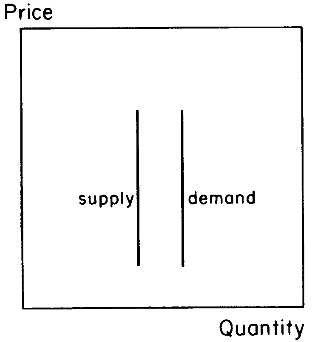
6.1. "Price-independent" supply/demand curves.
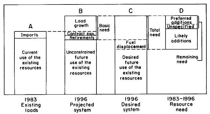
6.2. Conceptual flow of the California Energy Commission's integrated assessments forecasting methodology. Source: California Energy Commission (1985a), p. 45.
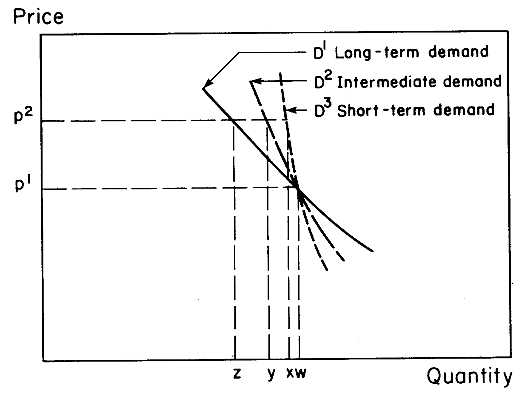
6.3. When the price of a commodity increases, demand declines. The demand reduction expands with the passage of time as buyers continue to adjust to the higher price.
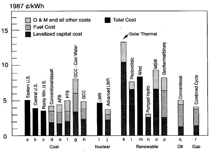
6.4. Costs and cost estimates for alternative electricity generation technologies. Based on data from Electric Power Research Institute (1986), pp. B-45 to B-105, a 30-year plant life, a 7% real interest rate, and a coal cost of $1.5l/million Btu, unless otherwise noted. (a-c) actual data on conventional coal plants in the Eastern, Central, and Rocky Mountain regions of the U.S., respectively. Source: Organization for Economic Cooperation and Development, Nuclear Energy Agency (1986), p. 11; (d) estimate for two 500-MW (net) conventional coal-steam plants with wet limestone flue gas desulfurization and a subcritical 2400 psi Steam system (40-year plant life, 65% capacity factor); (e) estimate for a 500-MW (net) AFBC plant (heat rate 10,000 Btu/kWh, 40-year plant life; (f) estimate for a 500-MW (net) PFBC plant (heat rate 8980 Btu/kWh); (g) actual data for the 103-MW (net) Cool Water GCC plant (65% capacity factor, fuel cost includes oxygen at 1.00¢/kWh and coal at $1.56/million Btu; the coal cost is likely to increase when the existing contracts expire). Source: Southern California Edison (1987); (h) estimate for a 500-MW (net) GCC plant (fuel cost includes oxygen); (i) actual data on conventional light-water nuclear plants in the Eastern, Central, and Rocky Mountain regions of the U.S. Source: Organization for Economic Cooperation and Development, Nuclear Energy Agency (1986), p. 11; (i) estimate for a 1100-MW (net) nuclear light water reactor plant to be available in 1995 (65% capacity factor); (k) estimate for a 150-MW solar thermal central receiver plant with dry cooling; (j) estimate for a 100-MW Solar Photovoltaic Central Station Plant; (m) estimate for addition of next 100 MW of wind power capacity (beyond 1985 levels), at 25% capacity factor. Source: Developed from Pepper (1985); (n) estimate for a pumped hydro storage system consisting of three 500-MW (net) plants; (o) estimate for a 45-MW (net) municipal refuse steam electric power plant (20-year plant life, 65% capacity factor); (p) estimate for a 50-MW (net) geothermal binary-cycle baseload plant (65% capacity factor); (q) estimate for a 500-MW (net) baseload residual oil-fired plant (heat rate 9,680 Btu/kWh, fuel cost $2.98/ million Btu); (r) estimate for a 390-MW (net) intermediate load, combined-cycle natural-gas-fired plant (heat rate 9,650 Btu/kWh, fuel cost $2.23/million Btu).
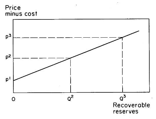
6.5. Recoverable reserves are a function of production costs and product prices.
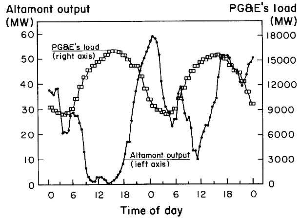
6.6. Comparison of the \ Pass wind farms output with PG&E system demand on peak demand days, July 17-18, 1984. Source: Smith, Steeley, and Hillesland (1984), p. 9.
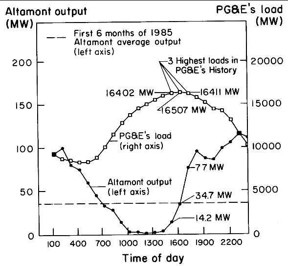
6.7. Comparison of the Altamont Pass wind farms output with PG&E system demand, July 9, 1985. Source: Smith, Steeley, Ilyin, and Hillesland (1985).
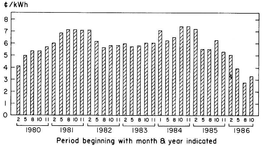
6.8. PG&E average avoided-cost rates for as-delivered energy, 1980-1986.
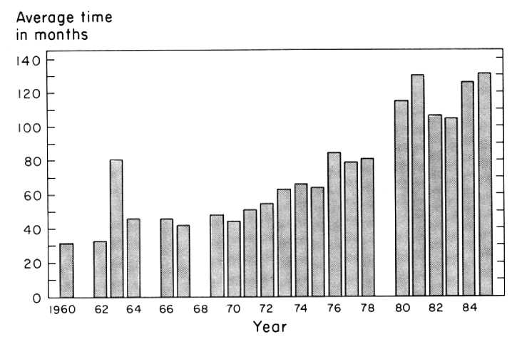
6.9. Length of construction period for U.S. nuclear power plants (interval from construction permit to full operation). Blanks indicate that no operating licenses were issued in the years shown. Source: Nuclear Regulatory Commission.
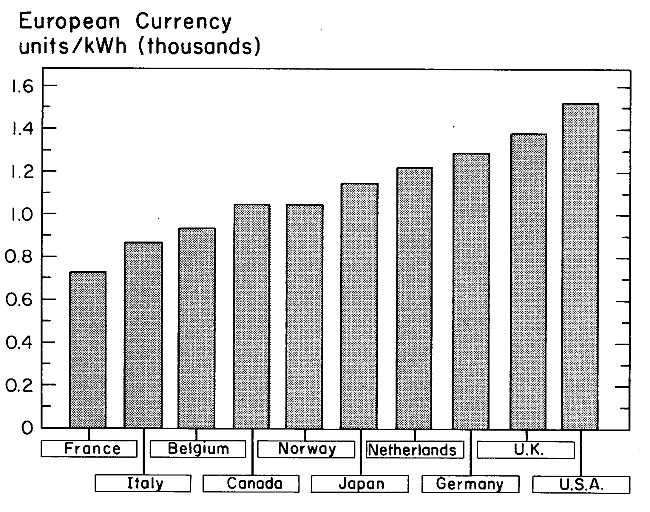
6.10. Capital cost of nuclear power plants, international comparison. Source: Organization for Economic Cooperation and Development, Nuclear Energy Agency (1983), p. 37.
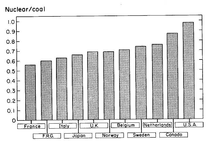
6.11. Ratio of nuclear-generated to coal-generated levelized electric power costs, international comparison. Source: Organization for Economic Cooperation and Development, Nuclear Energy Agency (1985), p. 37.
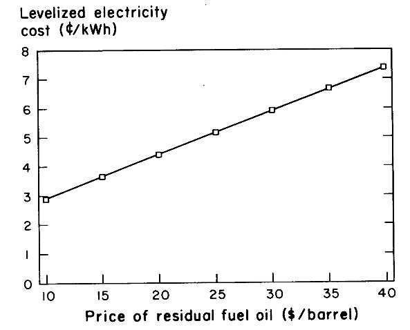
6.12. Cost of residual oil-fired electric power as a function of fuel price.
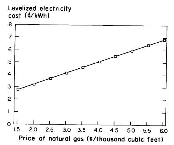
6.13. Cost of natural-gas-fired electric power as a function of fuel price.
SEVEN
An Economic Evaluation of the Costs and Benefits of Diablo Canyon
Alan J. Cox and Richard J. Gilbert
I. INTRODUCTION
Diablo Canyon is a 2,190-megawatt (MW) two-unit nuclear generating station located on the central coast of California and owned by Pacific Gas and Electric Company. Construction of the plant began in 1966 with units 1 and 2 scheduled for completion in 1972 and 1974. The original total cost was anticipated to be about $1 billion (1985 dollars). In 1971, as the first unit was nearing completion, Shell Oil announced the existence of a major geologic fault that ran as close as three miles to the reactor site. Evidence that the fault had the potential to generate earthquakes of greater magnitude than those that the plant had been designed for induced the Nuclear Regulatory Commission to revoke PG&E's operating license pending redesign of the plant. The Three Mile Island accident resulted in further redesign requirements. As these changes were being implemented, mistakes were made in drawing up designs and plans for construction, mistakes that were finally uncovered in 1981, when redesign was thought to be close to completion. Total cost, including allowance for funds used during construction (AFUDC), was projected to be $2.4 billion at that time. The final book cost, by the time mistakes had been corrected and the plant brought on-line, was more than double that amount.
With a book cost at completion of $5.67 billion, the Diablo Canyon nuclear power plant is one of the most expensive projects, if not the most expensive project, ever undertaken in the state of California. This chapter describes an analysis of the costs and benefits of Diablo Canyon.
From a purely economic perspective, most of the costs of units 1 and 2 of Diablo Canyon are sunk, and any comparison with other electric power alternatives should consider only the plant's present and future costs· However, noting the importance of total costs in regulatory proceedings, this chapter examines the costs and benefits of Diablo Canyon from 1985 and from earlier dates, acting as if it were possible to go back in time. The main question asked is whether the costs of Diablo Canyon could have been justified by the savings in expenditures on other sources of power made possible from the electricity produced by the plant.
The first section of the chapter poses this question from the approximate date at which unit I of the plant was completed. The total costs of Diablo Canyon units 1 and 2 are compared with the costs of electricity generated with oil and gas. In the second section of the chapter, the analysis is undertaken from an earlier date, chosen somewhat arbitrarily to be 1978. The question asked there is: Given the expectations that were current in 1978 regarding the costs and benefits of building a plant to displace fossil fuels, did it make economic sense to build the plant?
In both sections, no distinction is made between costs that are sunk and costs that can be recovered if Diablo Canyon is replaced by alternative sources of power. But any conclusion regarding the relative costs of Diablo Canyon must be tempered by the reality of those costs that are sunk and therefore must be paid whatever course of action is pursued. The third section looks specifically at the problem of sunk cost. In this section we compute the levelized cost of Diablo Canyon for each year of its construction, omitting all capital costs that have already been invested in the plant. (The assumption is that all incurred capital expenditures are not recoverable.)
By 1985 nearly all of the $5.67 billion (in nominal dollars) spent on Diablo Canyon units 1 and 2 was sunk. Omitting these costs, Diablo Canyon is clearly more economical than oil and gas and probably undercuts any alternative source of power for which costs have not been sunk.1 A different question, which again requires the luxury of hindsight, asks whether, during the recent history of the construction of Diablo Canyon, it would have been economically efficient to abandon the plant. The question is whether the levelized costs of Diablo Canyon, omitting sunk costs, exceeded the costs of alternative sources of power.
These assessments require assumptions about expectations of future costs. The assumption used in this paper is that the actual incurred costs
of Diablo Canyon could have been anticipated. Although this implies remarkable clairvoyance, it provides a reasonable bound on the value of the plant during the course of its construction.
A conclusion of this study is that even if the cost overruns for Diablo Canyon had been anticipated, at no time after 1974 was it economically efficient to abandon the plant given the base case forecast for oil and gas prices. Even with oil and gas prices corresponding to levels in 1986, the latest abandonment date is about 1981.2 More optimistic expectations about the total costs of Diablo Canyon would only strengthen the conclusion that some point between 1974 and 1981 was the latest date at which the plant could have been abandoned for economic reasons based on the value of fuel displaced. The conclusion is strengthened still further given the prevailing prices for fuel oil in world markets at that time.
The abandonment criterion used here is a comparison of levelized nonsunk costs. This criterion ignores the financial conflicts between stockholders and customers that arise from utility regulation. For example, stockholders may not be reimbursed for investments that are sunk in abandoned plants, which may make management reluctant to abandon a project. Customer revenues have to cover all utility costs without distinguishing between those costs that are sunk and those that are not. Thus customers may want to abandon a plant even if abandonment is not economically efficient when sunk costs are taken into account.3 Put another way, the conclusions about the abandonment decision for Diablo Canyon in this paper address the collective interest of stockholders, customers, and taxpayers, but the conclusions may not be consistent with the individual interests of any party.
The analysis in this paper does not deal with the complexities of electric utility ratemaking. The intention of this analysis is to include in the cost of the plant only those items that represent actual expenditures on scarce economic resources. Items such as taxes, which represent money transfers from one party to another, are excluded. As a consequence, the computations do not comply with tax or accounting conventions undertaken in typical regulatory proceedings.
The magnitude of the benefits from the Diablo Canyon plant is uncertain. Our study indicates that under fuel price assumptions used as the base case for this analysis, the total nominal cost of the project exceeds the value of the oil and gas displaced by the operation of Diablo by about 15%. However, the replacement cost of the nuclear facility estimated in
constant dollars is more than 30% greater than these oil and gas savings. When the project costs and benefits are viewed from dates before completion of units 1 and 2, the project's forecasted benefits exceed total incurred and forecasted costs. Most important, by 1974 the anticipated costs, in constant dollars, of finishing and operating the Diablo Canyon plant (excluding sunk costs) were lower than the base case forecasted costs of operating fossil-fuel-fired alternatives. Even if oil and gas prices are much lower than our base case assumptions and the actual costs of Diablo Canyon were fully anticipated, it was not economically efficient to abandon the plant later than early 1981. Thus by no later than 1981 the sunk costs of Diablo Canyon were large enough, relative to total costs, to justify continuing the project until its 1985-1986 completion date.
II. COSTS AND BENEFITS OF DIABLO IN 1985
Calculating the Costs of Diablo Canyon
Table 7.1 reports various estimates of the costs of units 1 and 2 of the Diablo Canyon plant as of January 1, 1985.4 The first two rows report the construction costs of both units in absolute terms and in dollars per kilowatt of capacity. These are expenses reported by PG&E to the California Public Utility Commission (CPUC) excluding taxes and with no adjustment to account for inflation during the construction period. Taxes are excluded because they represent a transfer of revenue from one party to another and our focus is on the economic resource costs of the project.
The economic cost of Diablo Canyon includes the foregone interest on capital that is invested in the construction of the plant. Because this money could have been invested elsewhere, the foregone income is a cost of construction. A regulatory approach to estimating the cost of foregone income is allowance for funds used during construction. AFUDC credits the utility with an estimate of the interest cost of debt and the return on equity used in construction. This credit accumulates in an AFUDC account, which, under traditional rate of return regulation, is added to the capital expenditures to determine the plant's contribution to the rate base when the plant is operational.
The plant's contribution to the rate base, R t , accumulates according to:
|
Rt +1 = (I + xt ) (Rt + It ) |
(7.1) |
where x t is the AFUDC rate and I t is the plant investment in year t. 5 Under traditional rate-of-return regulation with AFUDC accounting, the utility receives no actual earnings on R t until the plant is operational.6 If the plant is completed in year T and no costs are disallowed, the contribution to the rate base is R r .
The AFUDC account in year t, A t , is the difference between R t and cumulative construction expenditures up to date t, K t For Diablo Canyon, projected totals corresponding to a 1986 completion date are
R1986 = $5.67 billion
K1986 =

and
A1986 = R 1986 - K 1986 = $1.96 billion
AFUDC alone accounts for about 35% of the total book cost of the plant.
These figures are in nominal dollars and do not accurately reflect the true replacement cost of the plant. To estimate the replacement cost of Diablo Canyon, we first converted the construction cost to 1985 dollars by dividing annual construction costs by the GNP price index (normalized to 1985). This gives a construction cost in 1985 dollars of $5.03 billion.
The conversion of AFUDC earnings to constant 1985 dollars is more complicated. AFUDC is a payment for foregone interest and, as such, includes compensation both for the real cost of capital and for anticipated inflation over the construction period. Thus any calculation of the "replacement AFUDC" would depend on the time path of replacement investment and the cost of capital over the construction period.
A "replacement AFUDC" can be calculated in 1985 dollars by converting actual investment expenditures to 1985 dollars and applying a real (no inflation) cost of capital to expenditures over the actual construction period. This is very similar to what is actually done in AFUDC accounting, except that actual AFUDC expenditures are in nominal (rather than constant) dollars, and the AFUDC rate corresponds to the nominal (rather than real) cost of capital.
Suppose that the operation date T is the base year for measuring the replacement value of the plant. An investment of I r t in year- T dollars makes a contribution to the rate base in year T equal to (the superscript r denotes real quantities)
 |
(7.2) |
where xr v is the AFUDC rate in year t used for the replacement value calculation.
The constant-dollar investment I r t is related to the nominal investment I t by
|
Ir t =  |
(7.3) |
where it is the rate of change of the cost index in year t . Combining equations (7.2) and (7.3) gives
|
d Rr T =  |
(7.4) |
In nominal dollars, the contribution of It to the (nominal) rate base in year T is
|
It |
(7.5) |
The contributions in equations (7.4) and (7.5) are equal, to a first-order approximation, if xt = x r t + i t in every year. In other words, if the nominal AFUDC rate equals the real rate plus the inflation rate for capital investment, the two methods for calculating the rate base differ only by terms of the order i t xr t The replacement cost calculation yields the higher value, but the difference shrinks if the rate base is compounded over shorter time periods and disappears for continuous compounding.7
In evaluating whether the AFUDC account correctly compensated investors for the opportunity cost of capital, the answer hinges only on the relation between x t and x r t + i t If they are equal, then to a first-order approximation
|
KT + A T = K r T + A r T |
(7.6) |
Using equation (7.6), the reported values for KT and A T ,and the calculated value for K r T gives (in billions of 1985 dollars)
ArT = 3.71 + 1.96 - 5.03 = 0.64
The real compensation for funds used to finance the construction of Diablo Canyon totals about $640 million when a replacement value is calculated in 1985 dollars.
Figure 7.1 shows values of A r T and R r T that would be calculated with reported investment expenditures converted to 1985 dollars using the GNP deflator and using the indicated real cost of capital for x r t in every year. An AFUDC compensation of $640 million in 1985 dollars corresponds to a real AFUDC rate of about 1.75%/year.
Table 7.2 shows AFUDC rates for Diablo Canyon imputed from PG&E reports in nominal and real terms (using the GNP deflator). The AFUDC rate that justly compensates investors for the use of their funds is equal to their real after-tax cost of capital. This may be approximated by the weighted average of the before-tax cost of debt (because debt is deductible against earnings) and the after-tax cost of equity capital, with the weights corresponding to the firm's debt-equity ratio. The real weighted average cost of capital (WACC) after taxes is shown in column 3 of Table 7.2. This exceeded the real AFUDC rate in every year. Investors were not compensated for foregone interest until after 1968.8 Since that time, the real AFUDC rate varied from a low of-2.84% in 1974 to a high of + 4.89% in 1984. Over the same period, PG&E's WACC varied from a low of 0.62% in 1975 to a high of 8.84% in 1985, with a geometric mean of 3.8% over the period 1966-1984. The average annual rate, weighted by the total investment in each year, was 5.75%.
The lower AFUDC rates can be rationalized by appealing to traditional regulatory practice with its lower risk for utility investors relative to the manufacturing sector. Recent events have upset this historical relationship. Nonetheless, it is our view that the implicit real AFUDC rate of 1.75% was not adequate compensation for foregone interest, and a figure of 3.0-6.0% would have been more appropriate. A value of 4.75% gives real AFUDC earnings of about $1.5 billion, in 1985 dollars.9 Adding this to the replacement value of capital investment ($5.4 billion, 1985 dollars) gives a total replacement value of the plant equal to about
$6.9 billion in 1985 dollars. The nominal dollar cost of constructing the plant is $2.3 billion.
Comparisons of the costs of the Diablo Canyon plant with other nuclear power plants can be misleading because the available cost data are in nominal dollars and therefore include the toll of inflation over the construction periods. With this important caveat in mind, a simple comparison of the numbers in Table 7.1 with data available for other nuclear generating stations indicates that the costs of Diablo Canyon are about average for reactors coming on line in the mid-1980s. Komanoff (1984) reports, for instance, that the average construction and AFUI)C costs for 34 nuclear projects he sampled is $3,123/kW in nominal dollars, over $500/kW (nominal dollars) greater than Diablo. The sample included 14 multireactor projects that are generally less expensive (per kilowatt) to build. For multiunit plants, the average nominal cost including AFUDC drops to approximately $2,240/kW, about $350/kW (nominal dollars) less than PG&E's costs for Diablo Canyon.
After removing the AFUDC component for each plant and converting all expenditures to constant dollars, Komanoff reports the average construction cost for all 34 plants to be $2,428/kW in constant 1985 dollars.10 Our estimate of the equivalent figure for Diablo Canyon is $2,295/kW. The Komanoff paper does not give enough information to estimate the average constant-dollar cost for multiunit plants excluding AFUDC, but his data show that the average would be in the range of $1,400/kW-$1,650/kW. The constant-dollar construction cost of Diablo is appreciably larger than the multireactor national average: 39 to 63% larger, depending on where the national average actually lies. Yet the nominal cost of Diablo, including AFUDC, is only 15% larger than the multireactor national average. Thus compared with national averages, Diablo Canyon is relatively expensive in terms of construction expenditures but relatively cheap in terms of AFUDC. It seems that the extremely low real rates used to compute AFUDC earnings make Diablo appear, on a book-value basis, to have been bought at a fairly reasonable cost. The cost saving is only illusory, because the low AFUDC rates mean that much of the interest costs of Diablo Canyon were paid by utility investors without adequate compensation.
Comparison of Costs and Benefits
To make comparisons of costs of electricity from Diablo and other sources available or potentially available to PG&E, consistent estimates
of the levelized cost of electricity must be made and compared with the value of displaced electricity that would have been produced by an alternative generating technology. Realistic alternatives to nuclear power include fossil fuels (coal, oil, gas), and the more exotic technologies of solar, wind, and renewable resources. Hydropower and geothermal are sufficiently limited in supply to make them unavailable as replacement sources of energy. Conservation also has been proposed as an energy source: the cost of investments required to reduce demand, or the cost of foregone consumption, are measures of the cost of making energy available through the conservation option.
In this time period, oil and/or natural gas (henceforth gas) is the energy source used in the PG&E system with the highest operating cost (which includes the cost of fuel, labor, and wear and tear on equipment). Given the current configuration of the PG&E electric power system, most of the power produced by Diablo Canyon will displace gas, and hence the value of this production is the cost of gas fuel and the operating costs of the gas-fired capacity. One can argue whether different supply planning decisions and/or different approaches to load management might have created a situation in which the marginal energy source for the system would be something other than gas. In addition, with the benefit of hindsight, the power from Diablo Canyon might have been produced with different technologies; perhaps coal or wind.
This chapter takes the existing PG&E system as a given and measures the value of energy displaced by Diablo Canyon based on the cost of existing power from displaced facilities. Specifically, we estimate the energy benefits of the Diablo system on the basis of payments made by PG&E to small power producers for electric energy. Diablo Canyon also will displace generating capacity that would have been necessary in the absence of the Diablo capacity. We use the cost of a new gas-fired steam turbine plant as a measure of the cost of future displaced electric power capacity.
Oil and gas are proven technologies with relatively short lead times. Whether these energy sources are cheaper than alternatives such as coal, solar, or conservation is a subject of heated debate. Nonetheless, taking oil or gas as the alternative energy source provides an upper bound on the value of electricity produced by Diablo Canyon.
The assumptions contained in the base case are presented in Table 7.3. The most important of these are that the real discount rate is 10%; the expected real rate of increase in the price of oil and gas is zero until 1988 and 3%/year thereafter; the average heat rate of plants that are displaced by Diablo is 11,300 Btu/kWh; and Diablo Canyon achieves a capacity utilization rate of 65%.
Our basecase heat rate (the rate at which the heat content of fuel is converted to electric energy) is based on estimates provided by the
CPUC. These estimates are made to establish the price that PG&E must pay small power producers for electric energy. Before Diablo came on line the annual average heat rate for marginal plants was 12,427 Btu/ kWh. After both reactors came on line the annual average is estimated to be 10,356 Btu/kWh. The figure that we use for the heat rate in our base case is an average of the pre- and post-Diablo heat rates, used in computing payments to small power producers. These heat rates are actually lower than the heat rates of the plants displaced by Diablo Canyon (Pacific Gas and Electric, 1984a).11
The fuel cost assumed for a gas plant is $19/barrel of oil equivalent (BOE). This is the CPUC's estimate (California Public Utilities Commission, 1985, p. 22) of the incremental cost of natural gas plus delivery cost in 1985. The actual cost of gas delivered to PG&E's plants in early 1985 was $31.32/barrel of oil equivalent (in January according to Federal Energy Regulatory Commission [FERC] filings), falling to $27.27/barrel of oil equivalent in August. Establishing an appropriate price for the alternative fossil fuel is complicated by the fact that the CPUC has mandated (through its G-55 rate) that PG&E must charge itself a premium rate for natural gas used to produce electricity. The base case of $19/barrel of oil equivalent attempts to correct for this premium, which is effectively a transfer between electricity and gas ratepayers.
Capital savings due to fossil fuel plants not required as a result of Diablo are also included. Lost Capacity is made up by the addition of 1,900 MW of capacity that is assumed to have been constructed in 1983 and one 300-MW plant brought on-line in 2004. The addition of the first of these plants is justified by the capacity shortage experienced by the utility in 1983-1984.12
The levelized cost of electricity is computed by dividing the total cost of the project by the lifetime production of electricity, discounted to the present. The total cost includes the construction and AFUDC earnings of the project charged as a single lump-sum payment at the end of the construction period. In addition, operating and maintenance costs are
calculated over the life of the project and discounted back to the first day of 1985. The same computations are made for the gas-burning alternative. For the purposes of the results reported in Table 7.4, the capital cost of Diablo is the reported value in nominal dollars.
Estimates of levelized costs are made on the basis of a variety of assumptions as indicated in Table 7.4. The results suggest that, based on reported nominal costs of Diablo Canyon and base case projections of oil and gas prices, the nuclear plant falls short of paying for itself as measured by the value of oil and gas displaced over its useful life. In the base case, the levelized value of displaced oil and gas is 6.79¢/kWh, whereas power from Diablo Canyon has a levelized cost of 7.75¢/kWh.
Of course, these results are sensitive to assumptions such as projected oil and gas prices, the choice of the discount rate, Diablo Canyon's capacity utilization rates, and the heat rate in fossil fuel plants that are displaced by Diablo Canyon.13 If gas prices are projected to increase by 6%/ year, electricity from Diablo Canyon will be cheaper over the life of the plant. However, a 6% increase in gas prices is not sufficient to push the benefits of the project above its costs when the benefits of future price increases are discounted at 12%. In addition, a cost of gas of $24/barrel oil equivalent (escalated at the base case rate) would also result in Diablo Canyon paying for itself in terms of displaced oil and gas. This price is significant because it approximates the cost of gas to PG&E in 1985. In all cases, the assumption of no real increase in the cost of gas results in a shortfall in the net benefits of the nuclear project.
Table 7.5 shows the sensitivity of the results to changes in the assumed heat rate under the base case assumptions. The heat rates indicated in Table 7.5 are, in declining order, PG&E's average heat rate from marginal plants before Diablo Canyon came on-line, our base case rate, PG&E's average gas-fired heat rate after both units of Diablo came online, and the heat rate of PG&E's most efficient gas-fired unit operating at its most efficient level of production (Pacific Gas and Electric, 1984a). Even at the highest rate cited, the cost of electricity from the nuclear plant is 0.49¢/kWh above the cost of the gas alternative when other parameters are at their base case values. Lower assumed heat rates merely reduce the measured benefits further.14
The cost of Diablo Canyon in the above analysis consists of the nominal dollar reports of the construction costs and of the payments into the AFUDC account. To compare the economic costs that would have been incurred had Diablo not been built with the economic costs of Diablo, it
is necessary to convert the nominal dollar costs of the nuclear project to constant dollars. We recalculated the cost of Diablo by adding to the 1985 dollar cost an AFUDC earning estimated with a real allowed rate of 4.75%. This raises the 1985 dollar cost of Diablo to $6.9 billion. The resulting levelized costs, under a limited set of assumptions, are presented in Table 7.6.
A comparison between Tables 7.4 and 7.6 reveals that, once these corrections are made, the costs of Diablo Canyon substantially exceed the estimate of the avoided costs of oil and gas under base case assumptions. The 8.83¢/kWh estimate for the cost of electricity from Diablo is 30% greater than the cost of gas-fired electricity. Even if the cost of oil and gas increases at 6%/year from 1988, the avoided costs will not justify the investment in Diablo Canyon.15
Avoided cost is the basis of the regulatory procedure that was implemented by the CPUC to determine the earnings that PG&E is allowed on its investment in Diablo Canyon (California Public Utilities Commission, 1985). Under this scheme the utility is allowed to collect revenues as if it were operating the generating stations that were displaced by the nuclear plant.
PG&E already purchases electricity from small power producers at a price that is based on its (short-run) avoided cost. In the first quarter of 1985, before the first unit of Diablo Canyon came on-line, the purchase price for electricity averaged 7.2¢/kWh, with a peak price of 8.6¢/kWh. At that time PG&E announced that it would pay, during the next quarter, an average of 6.3¢/kWh if Diablo Canyon did not come on line and 5.6¢/kWh if it did, with peak prices being 7.4 and 6.4¢/kWh, respectively (Pacific Gas and Electric, 1985, Table E). The computed prices are biased upward in that they include the G-55 gas price surcharge but are biased downward by their exclusion of a capacity price. Payments made in the winter months also tend to be higher. The PG&E purchase prices again indicate that the benefits of Diablo Canyon fall short of its book value when measured against payments that the utility would have to make in the absence of the project.
The results presented in Tables 7.4 and 7.5 indicate the avoided costs that would be applied to Diablo Canyon under our assumptions. In general, the results indicate that payment to PG&E on the basis of avoided cost should allow the company revenues that would fall about 15% short of the total nominal cost of the nuclear plant. The CPUC (1985) report also provides estimates of annual revenue that PG&E would be allowed
to collect under an avoided-cost scheme. We have incorporated the CPUC assumed cost of gas of about $19/barrel of oil equivalent in our base case. Under the CPUC assumptions this price declines substantially until 1990 but increases at a high rate in the 1990s. Overall, their forecasted gas prices are equivalent to ours when discounted and averaged over the life of the plant. However, the CPUC assumptions differ from ours in a few notable areas. The CPUC heat rates for gas plants16 average about 9,500 Btu/kWh. Capacity credits, on the other hand, are based on the cost of cheap, but inefficient, gas turbine capacity, whereas ours are based on the cost of steam-driven generators. Finally, the CPUC assumes a 60% capacity factor. The total effect of these differences in assumptions results in a CPUC estimate of the avoided cost of Diablo Canyon being about two-thirds of our base case estimate. In fact, their estimated total payment (on a levelized basis) is about 3.8¢/kWh, about 56% of ours. This includes a payment for energy savings that implies a levelized cost of fuel of $14.20/barrel of oil equivalent, reflecting the considerable amounts of geothermal, other nuclear, and purchased energy that the CPUC estimates will be displaced by Diablo Canyon.
At a 10% real discount rate, the present value of payments to PG&E for the avoided cost of electricity displaced by the project is $4.13 billion under the CPUC scenario. Subtracting the nuclear plant's operating costs allows about $1.7 billion to pay for the capital invested, leaving $4.0 billion of the book value of the plant to be paid by stockholders and taxpayers (through tax deductions of losses). Of this, between $1 billion and $1.5 billion will be borne by PG&E's stockholders, depending on the tax regime during the plant's life. Under our base case assumption, the total cost will exceed total benefits by about $1 billion with about a quarter to a half billion of that paid by stockholders. In the next section we analyze whether such a shifting of the costs of Diablo Canyon from ratepayers would be justified on the basis of expected costs and benefits rather than on the basis of what actually transpired.
III. DIABLO CANYON VIEWED FROM 1978
Our base case results indicate that the costs of the Diablo Canyon nuclear plant exceed its benefits by a significant amount. PG&E's shareholders would be better off had the plant not been built even if the book value of the plant is recovered. Customers may be better off if only the book value is recovered and oil and gas prices rise considerably. These results are not surprising, considering the huge cost overruns, long delays, and considerable softening of oil and gas prices.
Would such a result have seemed likely in the late 1970s when it became apparent that Diablo Canyon would not operate on time and on budget? The question here is whether predictions of future oil and gas prices that were commonplace in the late 1970s justified further construction on the nuclear project, given the realized costs.
This question was examined by estimating levelized costs of electricity generated by both Diablo Canyon and a fossil fuel alternative, always discounting back to 1978 but allowing the nuclear project to come on-line in 1979, 1981, 1983, or 1985. The costs of Diablo Canyon are evaluated as replacement costs in constant dollars rather than the nominal dollars reported by PG&E, with AFUDC estimated on the basis of a 5% real rate of return. This clearly raises the measured cost of electricity from the nuclear plant.
One set of results is presented in Figure 7.2. The line labeled Cost 1 represents the levelized replacement cost of electricity from Diablo had it come on-line in the year indicated and had no further expenditures been necessary after the on-line date. The cost of the plant is assumed to be equal to the replacement cost of what had actually been spent on Diablo by that year measured in constant dollars, including the estimated AFUDC.
The levelized costs of electricity represented by Cost 2 is equal to Cost 1 plus the replacement cost of the additional investment that was actually made to complete the project after the year in which the project is assumed to come on-line. This additional amount does not include AFUDC. For instance, had the first unit come on-line in 1981, the levelized cost of electricity from Diablo would include all the expenditures that were made in the years 1981-1986 but none of the AFUDC earned in those years. Cost 2 is an approximation of what the real cost of Diablo Canyon could have been if the plant had been completed on an earlier time schedule. Some proportion of the distance between Cost 1 and Cost 2 could be thought of as an indication of the costs due to changes in the design of the project made since 1978.
The line labeled "average cost of oil and gas" is the forecasted levelized cost of electricity from a fossil fuel facility, including the capital costs necessary to replace Diablo Canyon. To be fully consistent with a view from 1978, some additional investment in capacity would have been made, as forecasts of the demand for electricity were much higher than the ones on which the previous simulations were based. The prices used for oil are those that were used in a California Energy Commission (CEC) report (1979). Thus the forecast of oil and gas prices corresponds to expectations held in about 1978. The average heat rate of the plants that are assumed to be displaced is 11,300 Btu/kWh.
The forecasts of the cost of oil by the CEC in 1979 reflect the relatively modest prices experienced before the 1978 increase, but they did predict sustained increases at a high rate toward the late 1980s. The predicted high prices account for the increasing per-kilowatthour benefits of the project. Given the high real increases predicted for oil prices in the CEC report, the levelized cost of electricity from Diablo Canyon is less than the cost of displaced oil and gas for every year of completion.
The scenario described by the CEC was commonly held in the late 1970s, with the forecasters of high prices finding considerable comfort in events of the Persian Gulf. Had the CEC scenario been borne out by events up to the present and/or should prices return to the predicted trajectory, the investment in Diablo Canyon would have been justified by the benefits in oil and gas savings.
The situation is considerably changed if predictions for the cost of oil are more in line with the experience of the last few years, as can be seen by examining Figure 7.3. Here the levelized cost of electricity displaced by Diablo Canyon is estimated on the basis of actual prices for oil to 1985, our base case forecast of $19/barrel of oil equivalent in 1986, and 3 percent real growth of gas prices after 1988. In this case the discounted present-value cost of electricity from Diablo rises above the discounted benefits between mid-1980 and 1983, depending on which cost estimate is used for the final cost of Diablo Canyon.
This does not imply that, from a societal point of view, PG&E should have abandoned the plant in 1977, because this calculation fails to separate sunk costs from the total costs of Diablo Canyon.
The traditional process of rate-of-return regulation for public utilities creates a divergence between the interests of private parties in the continuation of investment in new plant and the societal consequences of the investment (see Chao, Peck, and Gilbert, 1984, and Zimmerman, 1985). The societal value of continued investment depends only on the benefits and costs of expenditures that are not yet sunk. A utility must finance all expenditures but is compensated, under traditional regulatory practice, only for plant that is entered into the rate base, which typically requires that the plant be completed and operational. Thus utility shareholders have a financial interest in seeing construction projects through to completion. In contrast, ratepayers may prefer to cancel a construction project if cheaper power is available from another source. The difficulty with this comparison is that the private costs to ratepayers include sunk costs, while the social comparison between alternative sources of power should include only those costs that are not sunk. Total costs are minimized by abandoning an unfinished project in favor of an alternative source of power only if the cost of the alternative is less, excluding all sunk costs associated with the unfinished project and the alternative.
If a plant is completed, sunk costs become a source of revenue for shareholders and a cost of service for ratepayers. Peter (the ratepayer) pays Paul (the stockholder). The total payment cancels and thus the total (societal) value of continuing investment should not depend on sunk costs. The divergence between private and societal considerations can be increased with changing expectations about the value of the completed plant. In the late 1970s, when fuel prices were increasing, the projected value of the Diablo Canyon plant reflected the high projected cost of oil and gas. Based on initial construction estimates, Diablo Canyon offered a high return relative to the projected value of displaced oil- and gas-fired generation. This can be seen by comparing Cost 1 (the initial cost estimate for Diablo) in Figure 7.2 to the average cost of oil- and gas-fired generation displaced, based on 1070 energy price projections by the CEC (California Energy Commission, 1979).17
As construction difficulties with the Diablo Canyon plant mounted, it became apparent by the mid-1080s that the final cost of the project would be closer to that indicated by Cost 2 in Figures 7.2 and 7.3. Figure 7.2 shows that Diablo Canyon is arguably cheaper then the value of displaced oil and gas if energy prices corresponded to the CEC projections. Of course, energy prices fell sharply during the 1980s. When the Diablo Canyon plant was nearing its completion date, the relevant cost of oil-and gas-fired generation displaced was as shown in Figure 7.3. Under actual construction costs corresponding to Cost 2, the total cost of the Diablo plant, including sunk costs, exceeded the cost of displaced oil and gas as early as 1980. Because ratepayers have to shoulder the total cost of the plant, once it becomes apparent that total construction costs will exceed the value of displaced oil and gas, ratepayers would be better off by calling for immediate abandonment of the plant with a total disallowance of all Diablo Canyon expenditures, and then turning to new construction of an oil- or gas-fired alternative. As we shall argue below, this does not mean that abandonment of Diablo Canyon, as implied by Figure 7.3, is the alternative that minimizes the cost of producing power.
IV. THE ECONOMIC IMPACT OF SUNK COSTS
Most of the $5.67 billion spent on Diablo Canyon could not be recovered if the plant were abandoned. They are sunk costs and therefore economically lost. The social calculus governing the relative economic efficiency of Diablo Canyon versus other generation alternatives should consider only those costs that are not sunk. Costs that are sunk cannot be saved by any course of action. Sunk costs must be borne whether or not the
plant is used or replaced by another. Hence they are best forgotten when considering the costs and benefits of competing alternatives. Abandoning Diablo Canyon could change the party that bears the sunk cost. For example, ratepayers might avoid some part of the Diablo Canyon sunk costs by refusing to allow the plant to be included in the rate base. But the sunk costs still would have to be paid, and their amount would be unaffected by the abandonment decision.
Given that most of Diablo Canyon's cost are sunk, it is not economically efficient to abandon the plant and replace it with an alternative source of power. For example, at the end of 1984, about $5 billion, or 88% of Diablo's nominal capital costs, were paid. Assuming that these costs are not recoverable, the levelized costs of Diablo that were not sunk at the end of 1984 were 3.91¢/kWh in 1984 dollars. This compares with oil and gas costs of 6.79¢/kWh in the base case and 5.59¢/kWh in the low oil and gas cost scenario.
Of course the 3.91¢/kWh figure ignores past expenditures that contribute almost 5¢/kWh to the total generating costs of Diablo Canyon when costs are based on replacement value. But these costs have been paid and cannot be recovered. They will continue to be a cost to society whatever policy choice is made and however that policy shifts the accounting responsibility for the costs of Diablo Canyon. They have become, in effect, part of the earth.
By 1984 the operating and capital costs of Diablo Canyon that were not sunk had become so small that the continued operation of the plant clearly dominated the cost of switching to oil and gas as alternative sources of power. Moving backward in time, one may ask at what date (if ever) did the costs of Diablo Canyon that were not sunk exceed the costs of electricity generated with oil and gas. As always, the answer depends on assumptions. The assumptions here are as follows:
1. At each point in time it was possible to forecast the actual future expenditures on Diablo Canyon.
2. For every year under consideration, future expenditures and AFUDC earnings (at 5%) on those expenditures are discounted back to that year using the base case assumptions for the discount rate. Electricity production is also discounted back to that year.
3. Operating and maintenance costs are as in the base case.
4. Oil and gas costs correspond to either the base case or a low scenario of $14/barrel in 1986 rising at a 3% rate and a lower heat rate of 10,300 Btu/kWh.
Assumption (1) is not intended to imply that the actual costs of Diablo Canyon were perfectly anticipated. Rather, this assumption is a useful one for analyzing the economic costs and benefits of the plants if the
events that occurred could have been predicted. Assumption (2) permits the use of each year in the history of Diablo Canyon as the reference year for evaluating costs and benefits. It allows us to turn back the hands of time and consider the Diablo investment decision during each year in the history of the plant. Assumptions (3) and (4) are the same used elsewhere in this study.
Assuming that benefits and costs were predictable masks an important dynamic element. Discussions as to whether to abandon the nuclear plant in the past would have to have been based on information available at that time. For instance, even our base case assumptions on oil prices would have been considered wildly optimistic in the late 1970s. Oil prices were much higher, and few would have predicted the potential impact of cogeneration on electricity supply and on marginal heat rates.18
The results, expressed in levelized, nonsunk costs, are shown in Figure 7.4. The two horizontal lines represent the levelized cost of electricity from gas-fired plants. The higher of the two is the result of base case assumptions. The lower line replaces the basecase fuel cost with gas at $14/barrel of oil equivalent and the base case heat rate assumption with 10,300 Btu/kWh. The levelized values of electricity from the gas alternative remain constant over the period because, although the costs are discounted by a smaller factor as we move closer to the startup date, the electricity production is being discounted by exactly the same declining factor.
The levelized cost of producing electricity from Diablo Canyon declines every year, however, because we are only considering the remaining investment and the AFUDC to be paid on that investment.19 Diablo's declining nonsunk costs are represented by the downward sloping line in Figure 7.4. The points at which this line falls below the horizontal line represent the last time it made economic sense to abandon the plant. For our base case assumption this occurred during 1974. Figure 7.4 indicates that even with the lower heat rate and price for gas, an abandonment decision based on the net value of displaced oil and gas would have to occur before 1981.
It would seem unlikely that depressed oil and gas prices of the late 1980s could be credibly maintained as an economic argument to abandon the Diablo Canyon plant in the mid-1970s to very early 1980s, when expectations of ever-increasing costs of oil and gas were commonplace. The jagged line labeled "actual oil prices" gives some indication of the
state of then-current information. It shows the cost of electricity generated from oil sold at the average cost of heavy oil delivered to U.S. electric utilities (Energy Daily, June 13, 1985). The costs are estimated assuming that the real cost of fuel was projected to rise by 1%/year. This projection is clearly too low for the period of oil price controls between 1973 and 1981. Most forecasters were also watching world oil prices as an indicator of long-term oil prices. The assumed heat rate is 10,300 Btu/kWh.
Given these oil price projections it seems clear that continuing to build the plant was the social welfare-optimizing decision after the early 1970s, even if the final cost of the plant was known. Of course, the non-sunk Costs were always thought to be much lower than those indicated by the downward sloping line of Figure 7.4.
It is appropriate to discuss the history of the Diablo Canyon project in the context of Figure 7.4. The discovery of the location of the Hosgri fault close to the Diablo Canyon site was published in 1971 and was brought to PG&E's attention over a year later. By that time the utility had spent over $300 million (nominal dollars) on the plant and had been allowed to earn $40 million in AFUDC. Almost four years were spent debating the likely size of an earthquake that Diablo Canyon might have to withstand. Finally, in May 1976 the Nuclear Regulatory Commission (NRC) ordered a redesign of the plant. By that time the expenditure on the plant, including AFUDC earnings, had risen to almost a billion dollars.
It has been estimated that the cost to redesign the plant to the new NRC specification was $600 million (California Public Utilities Commission, 1987). However, before the plant came on-line new changes were ordered as a result of the Three Mile Island accident. These changes were estimated to cost $400 million. At the same time domestic costs for fuel oil were climbing rapidly. The low costs to finish the plant clearly indicate that, on a nonsunk cost basis, it was appropriate to complete the plant.
The last major milestone in the history of Diablo Canyon before completion occurred in late 1981 with the discovery of a major construction error, the "mirror image" problem. This discovery led to the uncovering of a large number of other errors. By that time a total of $2 billion had been spent. The final cost of the plant was becoming clearer, and the availability of alternative nonutility-owned sources of supply was better understood. At the same time world prices for oil were peaking at well over $30 a barrel. If low heat rates and the collapse of oil prices could have been confidently predicted, abandonment might have been appropriate. But as shown in Figure 7.4, in 1981 these nonsunk costs were
quite comparable to the value of displaced oil- and gas-fired generation at the low fossil fuel cost, and therefore abandonment of the Diablo Canyon plant in 1981 would have been a very close call.20
V. CONCLUSION
Estimates of the costs and benefits of Diablo Canyon indicate that the projected benefits of the project fall short of its costs when those costs are evaluated on the basis of either the plant's book or replacement value. The value of displaced electricity, assuming oil and gas prices that seemed reasonable when the plant first came on-line, exceed the book value of the plant. The benefits of the project will improve substantially if PG&E can maintain a high rate of utilization of the plant, if oil prices increase, or if unanticipated increases in electricity demand drive up the heat rate of marginal plants.
The net benefits of Diablo Canyon plummet when the projected value of displaced energy is compared with the replacement cost of capital invested in the plant. The replacement value of the plant is about $6.9 billion in 1985 dollars. The replacement value of construction expenditures is $5.03 billion in 1985 dollars, compared with a book value of $3.71 billion. Although our estimate of the replacement AFUDC is about the same as the reported AFUDC for Diablo Canyon, the latter is in nominal dollars and the implied compensation rate for foregone interest is less than the opportunity cost of capital. In real terms, the implied AFUDC rate for Diablo Canyon has averaged only about 1.75%/ year. This suggests that (all else equal) a substantial portion of the costs of Diablo Canyon have been underwritten by the shareholders of PG&E through inadequate compensation for foregone interest.
The dismal outlook for the net benefits of Diablo Canyon is a product of recent low oil and gas prices and the high opportunity cost of funds during the project's long construction period. Using forecasts of oil and gas prices developed in 1978 (after the 1973-1974 oil embargo but before the revolution in Iran), the benefits of Diablo Canyon exceed its replacement cost (and a fortiori exceed the anticipated replacement cost of the plant).
One can pose the question of whether at any time during the construction of Diablo Canyon it was economically rational to abandon the plant. If all of the cost overruns and the fluctuating oil prices could have
been predicted, the plant should never have been started. But information about both the high cost of the plant and its uncertain benefits developed over many years, and during this time more and more of the plant's total capital costs were irrevocably expended. Our analysis shows that, taking these sunk costs into account, by early 1074 the projected economic benefits outweighed the future costs of the plant using our base case assumptions, even if the large cost overruns could have been perfectly anticipated. Thus by 1074 purely economic considerations justified continued investment in Diablo Canyon. At gas prices of $14/barrel of oil equivalent and assuming an average incremental heat rate lower than our base case assumption, such a decline would have to have been anticipated by early 1081 to justify abandoning the plant on economic grounds.
REFERENCES
California Energy Commission (1979). Energy Futures for California: Two Scenarios, 1978-2000 . P102-79-016. Sacramento.
California Energy Commission (1985). The 1985 Electricity Report: Affordable Electricity in an Uncertain World . Sacramento.
California Public Utilities Commission (1985). "Diablo Canyon Nuclear Plant Value-Based Pricing Proposal."
California Public Utilities Commission (1987). "Review of the Costs of PG&E's Diablo Canyon Nuclear Power Plant Project and Recommendations on the Amount of Costs Reasonable for PG&E to Recover From its Customers." San Francisco, Public Staff Division.
Chao, H. P., R. Gilbert, and S. Peck (1984). "Customer and Investor Evaluations of Power Technologies: Conflicts and Common Grounds," Public Utilities Fortnightly , Vol. 113, No. 9, pp. 36-41.
Cox, A. J. (1978). "An Economic Evaluation of the Use of Wood Wastes to Generate Heat and Electricity at Pulp and Paper Mills in British Columbia." Vancouver: University of British Columbia, Resources Paper No. 20.
Helliwell, J. F., and A. J. Cox (1979). "Electricity Pricing and Electricity Supply: The Influence of Utility Pricing on Electricity production by Pulp and Paper Mills." Resources and Energy , Vol. 2, pp. 51-74.
Komanoff, C. (1984). "Assessing the High Costs of New Nuclear Power Plants." Public Utilities Fortnightly , Vol. 114, No. 8, pp. 33-38.
Pacific Gas and Electric Company (1984a). "Common Forecasting Methodology—V, Electric Supply Plan Forms," 1984-2004. Revised Submission.
Pacific Gas and Electric Company (1984b). Prepared testimony of Stephen P Reynolds.
Pacific Gas and Electric Company (1985). "Cogeneration and Small Power Production Quarterly Report," First Quarter, 1985.
Palmer, R. E., and R. R. Bum (1984). "Updating of Decommissioning Cost Estimates." In Transactions of the American Nuclear Society , Vol. 46, pp. 561-562.
Thermo Electron Corporation (1976). "A Study of Inplant Electrical Power Generation in the Chemical, Petroleum Refining and Paper and Pulp Industries." Washington, D.C.: Federal Energy Administration.
Zimmerman, M. (1985). "Regulatory Treatment of Abandoned Property: Incentive Effects and Policy Issues." Working Paper of the Graduate School of Business Administration. East Lansing: University of Michigan.
|
TABLE 7.1 |
||
|
Cost ($ in billions) |
Cost/kW ($/kW) |
|
|
Construction Costs Only |
3.71 |
1,696 |
|
Allowance for Funds Used During Construction |
1.96 |
895 |
|
Total Cost |
5.67 |
2,591 |
|
a NOTE: Dollar amounts in nominal dollars. |
||
|
TABLE 7.2 |
|||
Year |
Calculated AFUDC Rate |
Real AFUDC Rate |
PG&E's |
|
1966 |
0.00 |
-2.82 |
5.30 |
|
1967 |
0.00 |
-2.91 |
4.77 |
|
1968 |
0.00 |
-3.94 |
4.26 |
|
1969 |
4.44 |
-0.54 |
3.81 |
|
1970 |
5.84 |
0.61 |
3.47 |
|
1971 |
5.65 |
0.81 |
3.48 |
|
1972 |
6.09 |
2.01 |
4.36 |
|
1973 |
6.00 |
0.00 |
3.58 |
|
1974 |
6.29 |
-2.84 |
1.50 |
|
1975 |
6.87 |
-2.04 |
0.62 |
|
1976 |
6.34 |
0.51 |
4.34 |
|
1977 |
7.07 |
0.73 |
3.70 |
|
1978 |
8.06 |
0.24 |
2.90 |
|
1979 |
8.19 |
- 1.20 |
2.16 |
|
1980 |
8.72 |
-0.99 |
2.62 |
|
1981 |
9.42 |
-0.08 |
4.28 |
|
1982 |
9.89 |
3.28 |
5.16 |
|
1983 |
9.19 |
4.68 |
6.27 |
|
1984 |
9.08 |
4.89 |
7.03 |
|
1985 |
4.88 |
3.27 |
8.84 |
|
ABLE 7.3 |
|
|
Real Discount Rate: |
10% |
|
Real Rate of Increase in Cost of Fossil Fuels |
|
|
1985-1988: |
0.0%/year |
|
After 1988: |
3.0%/year |
|
Average Heat Rate of Fossil Fuel Plants Displaced |
11,300 Btu/kWh |
|
Annual Real Increase in Operating and Maintenance |
|
|
Costs of a Plant |
1.5%/year |
|
Operating Cost of Diablo |
|
|
Fuel: |
1.4¢/kWh |
|
Nonfuel variable and fixed: |
0.8¢/kWh |
|
Decommissioning Cost of Diablob |
$164,000/MW |
|
Cost of Gas-Fired Plant |
$820/kW |
|
Operating Cost of Oil and Gas Plant |
|
|
Fuel: |
$19.00/BOEc |
|
Nonfuel variable and fixed: |
0.4¢/kWh |
|
Capacity Utilization Rate for Diablo Canyon Units 1 and 2: |
|
|
1st year |
40% |
|
2nd year |
55% |
|
3rd-25th years |
65% |
|
26th-27th years |
60% |
|
28th-29th years |
55% |
|
Last year |
50% |
|
a NOTES: Currency units are in 1984 dollars and cents. |
|
|
TABLE 7.4 |
|
|
Levelized Cost |
|
|
Base Case |
|
|
Diablo Average Capital Cost (including AFUDC) |
5.43 |
|
Diablo Average Total Cost |
7.75 |
|
Value of Oil and Gas Saved |
5.17 |
|
Including Capital Savings |
6.79 |
|
Base Case With No Real Increase in Oil and Gas Prices |
|
|
Oil and Gas Savings, Including Capital Savings |
5.82 |
|
Base Case With 6%/Year Real Increase in Oil and Gas Prices |
|
|
Oil and Gas Savings, Including Capital Savings |
8.26 |
|
Base Case With $14/BOE Gas |
|
|
Oil and Gas Savings, Including Capital Savings |
5.59 |
|
Base Case With $24/BOE Gas |
|
|
Oil and Gas Savings, Including Capital Savings |
7.99 |
|
Base Case, Discounting at 8.5% |
|
|
Diablo Average Capital Cost |
4.73 |
|
Diablo Average Total Cost |
7.06 |
|
Value of Oil and Gas Saved |
5.28 |
|
Including Capital Savings |
6.68 |
|
With 6%/Year Real Increase in Fossil Fuel Prices |
|
|
Value of Oil and Gas Saved |
6.94 |
|
Including Capital Savings |
8.34 |
|
Base Case, Discounting at 12% |
|
|
Diablo Average Capital Cost |
6.44 |
|
Diablo Average Total Cost |
8.74 |
|
Value of Oil and Gas Saved |
5.05 |
|
Including Capital Savings |
6.97 |
|
With 6%/Year Real Increase in Fossil Fuel Prices |
|
|
Value of Oil and Gas Saved |
6.30 |
|
Including Capital Savings |
8.22 |
|
With 0%/Year Real Increase in Fossil Fuel Prices |
|
|
Value of Oil and Gas Saved |
4.21 |
|
Including Capital Savings |
6.13 |
|
TABLE 7.5 |
|
|
Base Case With Average Heat Rate of Oil and Gas Alternatives Assumed To Be: |
Levelized Cost (1985 ¢/kWh) |
|
12,400 Btu/kWh |
7.26 |
|
11,300 Btu/kWh |
6.79 |
|
10,300 Btu/kWh |
6.38 |
|
9,400 Btu/kWh |
6.00 |
|
TABLE 7.6 |
|
|
Levelized Cost (1985 ¢/kWh) |
|
|
Base Case |
|
|
Diablo Average Capital Cost |
6.51 |
|
Diablo Average Total Cost |
8.83 |
|
Base Case, Discounting at 12% |
|
|
Diablo Average Capital Cost |
7.72 |
|
Diablo Average Total Cost |
10.02 |
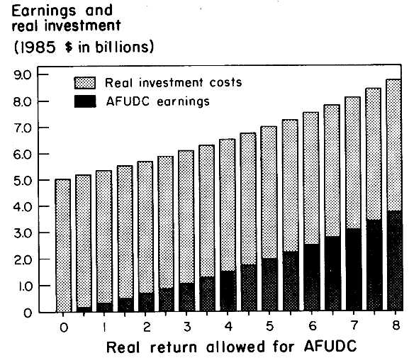
7.1. Replacement cost of Diablo Canyon.
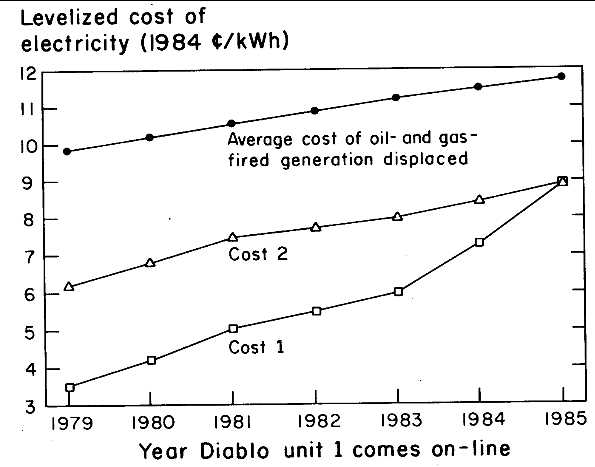
7.2. Effect of delay from 1978: comparison with the cost of displaced fossil-fired generation at CEC-forecasted average oil prices (California Energy Commission, 1979). An average heat rate of 11,300 Btu/kWh is assumed for the plants displaced.
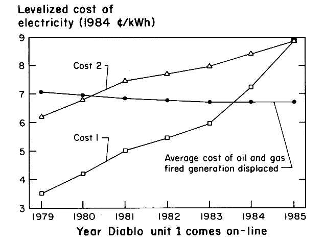
7.3. Effect of delay from 1978: comparison with the cost of displaced fossil-fired generation at actual oil prices. An average heat rate of 11,300 Btu/kWh is assumed for the plants displaced.
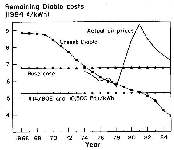
7.4. Levelized cost of electricity excluding Diablo's sunk cost. The curve labeled "actual oil prices" is the cost of electricity produced from heavy oil at the average price delivered to U.S. electric utilities and a heat rate of 10,300 Btu/kWh.
EIGHT
Residential Energy Conservation Standards, Subsidies, and Public Programs
John M. Quigley
I. INTRODUCTION
The dramatic increase in world energy prices in the early 1970s led to a variety of painful market adjustments and to the imposition of regulatory policies intended to stabilize domestic prices, to allocate energy resources on more equitable grounds, and to improve the technical engineering efficiency of energy utilization. Fuel prices were controlled, energy was allocated regionally and was rationed by queues, and "conservation" took on patriotic significance.
An important object of conservation was the energy used in residences; fully one-fifth of total U.S. energy demand arises from the requirements to heat, cool, light, or to provide hot water in residential dwellings. Thus, to an important extent, the overall impact of substantial increases in the level and variation in world energy prices on the economy depends on the potential for energy conservation in the residential sector of the U.S. economy. Even modest relative savings in energy consumption can lead to large absolute savings in energy and can increase its availability for industry or for the commercial sector of the economy.
This chapter reviews government policies designed to promote conservation of energy in the residential sector. By conservation I mean reductions in energy consumption from the levels that would otherwise be observed in the market, given prices and incomes, production processes, and forecasts of future conditions. The counterfactual is based on expectations about the actual operation of the market, not necessarily the idealized market of the economics textbook or the engineering caricature obtained by neglecting the possibilities for substitution in production and consumption.
The analysis provides a parallel treatment of federal tax credit and regulatory policies and those adopted by the state of California. The federal-state comparison is especially fruitful. The California programs of residential tax credits and building standards were similar to but much more ambitious than those of the federal government. I begin with a discussion of government grant and tax credit policies designed to encourage the direct substitution of capital for energy in the construction or retrofit of dwellings. Section II below discusses policies of the federal government and of the state of California. Section III expands the discussion to include a variety of incentive programs authorized, directed, or mandated by state regulatory agencies but undertaken and implemented by public utilities themselves.
Section IV considers a variety of mandated standards for residential construction, regulations that require compliance with specific mandates governing inputs or energy usage. Section V summarizes the expectations about future energy prices that may have motivated some of these policies, at least ex ante.
II. RESIDENTIAL WEATHERIZATION AND ALTERNATIVE ENERGY PROGRAMS
The oil crisis resulting from the OPEC oil embargo of 1973-1974 shifted the emphasis of federal energy policy toward the recognition of conservation as an explicit policy goal. This change can be seen in the language of Project Independence, proposed in November of 1973 by the Nixon Administration, and in the content of laws passed in the mid-1970s to promote conversion to alternative energy sources.1
The zenith of this change in federal energy policy was the National Energy Act of 1978 (PL 95-618), which introduced an explicit policy of energy conservation. Indeed, the articulation of this policy was a principal
goal of the act itself, and the residential sector of the economy was the principal object of the policy. The government contended that residential buildings were inefficient and wasted a substantial amount of energy, and thus the new policy had considerable scope for reducing energy use by increasing conservation in the residential sector. The National Energy Act introduced a federal system of income tax credits (subsequently amended by the Crude Oil Windfall Profits Act of 1980, PL 96-223). The Energy Act of 1978 contained a variety of energy-conserving provisions: the "gas guzzler" tax, incentives for van pooling, and a variety of business energy tax credits. The principal tool of federal policy introduced by the act, however, was a system of personal income tax credits.
Direct Federal Subsidies
Before the introduction of these tax credits, however, the federal government had undertaken a direct program to increase the insulation in dwellings occupied by low-income households. The Energy Conservation in Existing Buildings Act of 1976 authorized the Department of Energy (DOE) to develop and implement a Weatherization Assistance Program (WAP) to assist in achieving a prescribed level of insulation in the dwellings of low-income persons. DOE's program regulations allow up to a maximum of $1,600 per dwelling for numerous weatherization measures, including caulking; weather stripping and repair; insulating attics, exterior walls, floors, and water heaters; modifying furnaces for greater efficiency; and installing storm windows and doors. Under this program, funds are distributed to the states for implementation and dispersal. In California, for example, program funds are allocated to the Community Action Committee of the California Department of Economic Opportunity. The committee evaluates grant proposals from local groups, subject to DOE eligibility guidelines. About 60 community action programs were being funded in California in 1984.
Through 1984, about $1.4 billion in federal funds had been allocated under this program. Through 1984, weatherization had been completed for about 1.4 million of the estimated 14.4 million dwelling units occupied by eligible low-income persons. In the same period for California, 66,000 of the estimated 1.35 million eligible units were weatherized.
After the second shock in energy prices in the late 1970s, the Low-Income Home Energy Assistance Program (LIHEAP) block grant was established. The act encourages the states to use the block grant to facilitate low-cost weatherization by low-income households. Federal requirements regarding the use of LIHEAP weatherization funds are minimal, and neither the act nor the regulations define low-cost weatherization. Therefore the program provides substantial flexibility for
states in designing their programs, including the establishment of cost and income eligibility within the limit set in the act.
Table 8.1 summarizes federal funding of these weatherization programs during the years 1982 through 1985. Direct federal expenditures for weatherization rose from $279 million in 1982 to $398 million in 1985; expenditures in California increased from $7 million to almost $14 million during the period.2 Section 155 of the 1983 Further Continuing Appropriations Act provided for the disbursement of up to $200 million in Petroleum Violation Escrow Account (PVEA) funds to each of the states. The states could use these funds to supplement the WAP and the LIHEAP, as well as for energy-related purposes other than residential conservation.
On March 6, 1986, the DOE released nearly $2.1 billion to the states, reflecting the settlement of oil overcharge litigation with the Exxon Corporation. California received $194.7 million from the PVEA account, or 9.4% of the available funds.
In addition to these weatherization programs, the federal government has provided modest subsidies to encourage solar energy investment through the Solar Energy and Energy Conservation Bank, which authorized the Energy Security Act of 1980. A total of $81.9 million has been appropriated to the bank for fiscal years 1982 through 1985.
Government Tax Credits
Compared with these direct-subsidy programs aimed at low income households, programs of tax credits aimed at upper income households have been quite large.
Federal Tax Credits. The system of residential energy tax credits authorized by the National Energy Act of 1980 included the following features:
First, a credit of 15% against federal income tax liability was permitted for up to $2,000 of qualifying expenditures on particular insulation and energy-conserving devices, including caulking, weather stripping, storm windows, furnace replacement burners, and so forth. The maximum credit allowed was $300, and the minimum that could be claimed was $10.
Second, legislation provided a credit for investment in equipment that uses renewable inexhaustible sources, such as solar, wind, and geothermal energy. The 1978 act provided for a 30% credit for the first $2,000 in expenditures and a 20% credit for the next $8,000 of investment up to a maximum of $2,200 in tax credit for investments in renewable
resources. When amended in 1980, the credit was increased to 40% of the first $10,000 in expenditures, up to a $4,000 maximum.
Third, these credits were nonrefundable, and they were subject to particular limitations. Certain alternative government energy subsidies did reduce the amount of the tax credit available in any year, but the energy credit could be carried forward until exhausted or until 1987. Significantly, the credit applied only to principal residences; hence, it excluded vacation homes, second homes, and so forth. Renters as well as homeowners could qualify.
Fourth, investments were required to be in new devices having useful lives of at least five years. A number of potential conservation devices were excluded from the credit, for example, wood-burning stoves and passive solar systems.
This extensive program of tax credits expired on December 31, 1985. Table 8.2 provides a summary of the provisions of the federal acts.
State Tax Credits. The system of California state energy tax credits was introduced two years before the federal program; since 1976 the state of California has enacted eight laws that authorize tax credits for investments in certain classes of energy-saving capital equipment in residential dwellings. Between 1976 and 1980, the state enacted four bills providing tax credits for solar and wind energy systems for dwelling units. The first of these, the so-called Alquist Bill (SB 218) adopted in 1976, provided solar energy tax credits for individual and corporate taxpayers. Taxpayers were permitted to claim a tax credit equal to 10% of the cost of acquiring and installing solar energy equipment for heating, cooling, or producing electricity in residential dwellings, up to a maximum credit of $1,000. The bill specified that the credit could be claimed only once between January 1, 1976, and December 31, 1980. This 10% tax credit remained in effect until September 1977, when new legislation (AB 1558) established a 55% tax credit, up to a limit of $3,000, for solar systems for single-family dwellings (including condominiums). This bill also extended eligibility to specific conservation measures installed in conjunction with a solar heating or cooling system.
For multifamily dwellings and for commercial or industrial buildings the 55% credit applied to investments up to $12,000 in total costs. In excess of $12,000, the credit was set at 25% of the cost without an upper limit. The bill specified that this credit would expire on December 31, 1980.
In 1978 the solar credit program was amended again (by AB 3623) to allow the builder or the developer of a new dwelling to claim the credit at the time of construction or to pass on the tax credit to the original purchaser of a new dwelling. Wind energy systems and the cost of ac-
quiring a solar easement were also made expressly eligible for the tax credit by the 1978 bill.
During the 1980 legislative session the California code was amended again to extend the expiration date of the credit to December 31, 1983, and to expand the 55% credit to include all residential applications rather than simply single-family dwellings. This bill also provided for successive reductions in the credits available for recreational or therapeutic solar energy water heating systems, from 55% in 1980 to 45% in 1981, to 35% in 1982, and to 25% in 1983.
Also in 1980 the California legislature passed California's first conservation tax credit (AB 2030). This bill permitted a taxpayer to claim a 40% credit for investments in conservation measures installed in dwellings or in other premises, up to $1,500 in credit. For conservation investments exceeding $6,000 and installed on premises other than dwellings, a credit of 25% was provided, again without an upper limit. The conservation tax credit became effective on January 1, 1981, and AB 2030 specified expiration dates varying from December 31, 1983, to December 31, 1986, depending upon the type of measure and the property affected.
In 1983 Governor George Deukmejian proposed the elimination of both the solar energy credit and the energy conservation tax credit programs. The legislature held separate hearings to consider the governor's proposal and ultimately included amendments in the state budget's "Trailer Bill," extending the credits for several years while at the same time reducing the credit level and eliminating the eligibility of certain measures. The solar and wind energy tax credits were extended through December 31, 1986, but the 55% solar tax credit was reduced to 50% beginning August 1, 1983. All tax credits for solar heating of pools and spas were eliminated as of August 1983. The measure also reduced California's 40% conservation tax credit to 35%, but extended eligibility for these tax credits until December 31, 1985. Finally, the bill provided that only one-half of available credits for certain measures could be claimed against 1983 tax liability, with the remainder carried forward against future tax liabilities.
Also in 1983 two additional bills, SB 298 and AB 2158, were enacted to revise the solar and conservation tax credit program. The former made three changes to the solar tax credit, retroactive to January 1, 1983. First, the amount of the tax credit for builders and developers who elected to claim the state tax credit (instead of passing it on to the original purchaser) was reduced from 25 to 15%. For solar energy systems that were also eligible for federal credit, the state credit was also reduced to 15%. The solar credit was simplified by removing a $12,000 minimum cost threshold for solar systems installed in premises other than
dwellings. Under the revision, all solar and wind systems in nonresidential properties were eligible for the 25% state tax credit. Third, the eligibility for tax credit of leased solar systems was expanded. The latter bill (AB 2158) removed the requirement that a taxpayer have a home energy audit provided and paid for by the local utility company as a condition of eligibility for certain categories of conservation measures: wall insulation, floor insulation, cooling fans, and heat pumps.
Finally, in 1985 two bills were enacted that reduced substantially the total amount of credit that could be claimed by taxpayers. These bills deleted provisions that link state tax credits to eligibility for federal credits. They also reduced the allowable credit as a fraction of total investment. Under the new law, solar credits for single-family residential dwellings were limited to 10% of the system cost regardless of the availability of federal credit, up to a maximum credit of $1,000. For multifamily residential construction, credits were limited to 5% of the total cost, with no maximum credit per unit. For commercial and industrial properties, solar credits were limited to 25% of the total system costs. Credits for wind energy were changed to be generally similar to solar credits. Solar and wind energy tax credits expired on December 31, 1985.
These bills also revised and reduced the state energy conservation tax credit program. For single-family residential dwellings, the credit was reduced to 10% of the cost of all qualifying systems, regardless of the availability of the federal credit. The maximum credit was reduced to $750. Eligibility for many of the qualifying items expired December 31, 1985; all others expired at the end of 1986. For multifamily dwellings, the state credit was reduced to 25% of total cost effective September 1, 1985, through December 31, 1985, and to 20% of total cost during calendar year 1986. Ail state tax credits under these programs expired on December 31, 1986.
Table 8.3 summarizes state programs for tax credits for solar, wind, and conservation investments.
Program Impacts
Individuals availed themselves of tax credits under these programs by including the relevant information on their personal income tax returns. U.S. taxpayers submitted form 5695 to the Internal Revenue Service; California taxpayers submitted form FTB3514 to the state's Franchise Tax Board. Thus a wealth of descriptive information about these tax expenditure programs is compiled, but not published, by agencies administering the tax code.
Tables 8.4 and 8.5 summarize unpublished data on the impact of federal credits for renewable energy sources and for energy conservation during the period 1978-1982. As reported in Table 8.4, qualifying in-
vestments in solar, geothermal, or wind energy sources increased from $115 million to $805 million from 1978 to 1982, and total tax expenditures under this program increased from $29 million to $322 million. Since 1980 about 80% of these tax expenditures were made to households earning more than $25,000 a year. The average tax credit per household varies directly with income and is 15 to 20 times as large for households earning $100,000 than for households earning $10,000 a year. Part D of the table indicates that the fraction of households claiming these credits is quite small. Only for the highest income households does it approach 1%.
The average investment in renewable energy sources made by those claiming the credit increased from $1,750 in 1978 to $3,500 in 1982; investments increase moderately with incomes. The average credit claimed by investors increased from $450 to $1,400. Credits per investor increase moderately with income.
Table 8.5 provides similar information for energy conservation tax credits. Qualifying investments under this program declined from $3.6 billion in 1978 to under $2.0 billion in 1982, and federal tax expenditures declined from $493 million to $292 million during this period.
The distribution of average tax credits by income class, reported in part C of the table, is regressive, but much less so than the credits for renewable energy sources. A much larger fraction of households claims credits under this program, but neither the average qualifying investment nor the average credit per investor varies much by income class.
For both the federal renewable energy and the conservation tax credit programs, the regressivity of benefits arises more from variations in the proportion of households claiming credits by income class than from variations in credits claimed per investor.
Similar information is available on the California tax credit programs for wind and solar energy investments and for energy conservation investments. Tables 8.6 and 8.7 provide information on the kinds of investments undertaken by households claiming these credits. Table 8.6 refers to the California Wind and Solar Energy Investment program. As part A of the table indicates, total claims for tax credits under this program increased from 16,800 household returns in 1978 to a high of 85,100 returns in 1980. In the most recent year for which data are available, 1983, over 57,000 state personal income tax returns claimed credit for investment in wind and solar energy. Part B of the table indicated the reported amount of wind and solar investment qualifying for the tax credit. The reported investment has steadily increased from $31.4 million in 1978 to over a half billion dollars in tax year 1983. During the first three years of the program, qualifying investments were heavily concentrated in the heating of swimming pools and recreational spas.
About half of the investments claimed during the years 1978-1980 were in those categories. When the law was amended to phase out the eligibility of these investments, the mix shifted rather rapidly. During the 1981-1983 period, qualifying investments in solar hot water systems more than tripled to $192 million, and investments in solar heating and air conditioning systems increased to $71.3 million. The most substantial increase, however, was in wind systems. The distribution of investments is noted in part C of the table. It indicates that about a third of the qualifying investments during the other period have been made in hot water systems, and an eighth in heating and air conditioning. In 1983 almost 46% of qualifying investment was made in wind systems.
Table 8.7 presents similar information for California Energy Conservation Tax Credits, which went into effect in 1981. The table indicates the number of claims, the value of the qualifying investments, and the distribution of those investments. As the table indicates, the number of households claiming the credit has been substantial, between 190,000 households and 240,000 households, or more than four times the number claiming wind and solar energy tax credits. The value of the qualifying investments is substantially less, however, varying between $195 million and $230 million. As the table indicates, insulation expenditures have made up about half of the total qualifying investments. Storm windows have increased from 6 to 15% of total investment and heating and cooling devices have increased from a smaller base. A little less than one-third of the total qualifying investment is claimed in multifamily dwellings (where it is not possible to identify the particular system that has been installed).
Tables 8.8 and 8.9 present information on these two state programs by income class. They are thus directly comparable to tables 8.4 and 8.5 for the federal programs. Table 8.8 refers to the distribution of solar and wind energy tax credits by income class. Part A of the table shows the distribution of qualifying investments made by households of varying income categories. Households with higher income tend, on average, to claim more in qualifying energy investments. Households in the higher income classes also report larger investments generally. In part, of course, this reflects the peculiar economic circumstances of those who report tax losses for state income purposes. Over time, it appears that the concentration of qualifying investments among households of the highest income classes has increased. By 1983, for example, $235 million of the $554 million in qualifying investments was made by households whose adjusted gross income was greater than $100,000. Similarly, over time the total tax credit has become both larger and more concentrated among households of higher incomes. Part B notes these trends; the total tax credit increased from $6.5 million in 1978 to $126 million in
1983. By 1983, $98 million of the $126 million aggregate credit was claimed by households whose incomes exceeded $50,000 per year. In fact, the tax credits generated by households with incomes greater than $100,000 per year exceeded all the credits distributed through the entire program two years previously. Part G of the table indicates that the average tax credit for households in the state has been relatively small, at least until 1983. The tax credit increases with the income of the households, and only for the highest income households is it a large number. By comparison, however, it should be noted that in 1985 the renters' tax credit for joint filers was $137 per year, and the credit for an additional personal exemption on California incomes taxes was $13 per year.
The fraction of households claiming the tax credit clearly increases with income, and for the highest income categories it is on the order of 2 to 6%. In 1982 about 2.5% of households earning between $50,000 and $100,000 claimed the tax credit; 2.18% claimed it in 1983. Of households earning greater than $100,000, 6.5% claimed a credit in 1982, and 5.9% claimed it in 1983. Part E of the table indicates the average qualifying investment made by households of different income classes. Again, the table reveals that for households that have made investments in solar and wind systems, the average level of the investment is rather high, ranging between $1,900 and $3,900 per year through 1981; it also increases with income. During 1982 to 1983, the level of investment by the highest income households increased substantially. The concentration of the credit in the highest income classes and the very large qualifying investments reflect the surge in investment in "wind farms" during the past few years. Finally, part F of the table shows the average credit claimed by those who claim tax credits. The credit varies between $350 and $1,000 for middle income households, but increases to $2,200 to $7,600 for the highest income categories.
Table 8.9 provides similar information for the California Energy Conservation Tax Credit program introduced in 1981. Part A of the table indicates the value of the qualifying investments in millions of dollars. In contrast to solar and wind energy tax credits, conservation investments do not increase as markedly with income. Neither, in fact, does the total tax credit, which has varied between $50 and $61 million during the period 1981-1983. Because the number of households claiming energy conservation credits is so much larger than those claiming solar and wind energy credits (as noted in part D of the table), the average credit per household in the California population is not too different by income class. Middle income households are five to ten times more likely to claim energy conservation tax credits that to claim wind and solar energy tax credits. As part E of the table indicates, the average
qualifying investment is substantially lower for energy conservation than for wind and solar, averaging on the order of $1,000 per qualifying investment. There is some tendency for investments to increase with income.
Finally, the average tax credit claimed per investor is also substantially lower than for solar and wind credits; it averages about $250 per claim. Again, there is a rather pronounced tendency for tax credits to increase with the income of households (again, with the exception of the very lowest adjusted gross income classes, which includes some very wealthy households). In the highest income classes, the average credit claimed per investor is between $270 and $650.
Evaluation
As the documentation in Tables 8.4 through 8.9 indicates, these subsidy programs have been quite expensive. They have also been extraordinarily regressive. General taxpayers have provided extremely generous subsidies to those in the very highest income classes. The economic rationale for these expensive and regressive programs appears quite weak. Attempts to justify these programs could be based on two different arguments.
First, consumers may be unable to evaluate appropriately the savings arising from investments in retrofit activities or to act upon that evaluation. A variety of engineering standards are routinely set to protect consumers from the consequences of their own ignorance, and these subsidy programs could be seen as a less draconian regulatory device. If consumers are, in fact, capable of calculating their self-interest, liquidity constraints could still prevent them from investing in appropriate retrofit technologies. In this latter circumstance, however, tax credit programs are likely to be inferior to revolving funds offering market rate loans for conservation investments.
Second, if consumers are neither ignorant nor capital constrained, their optimizing decisions regarding conservation investment may be based on energy prices that do not represent scarcity or societal costs. In particular, if energy prices are controlled or regulated by other policies, then even informed consumer choices would in general lead to underinvestment in energy-saving residential capital.
Other economic arguments are sometimes made to justify investments in alternative energy sources, such as solar heating systems and wind farms. These rationalizations are typically based on some variant of the infant industry argument; public investments will facilitate scale economies that will reduce investment costs and hence energy costs to consumers over some longer run. With efficient energy prices, of course,
there is no more reason to subsidize the exploitation of these scale economies using public funds than to subsidize the exploitation of scale economies in the automobile industry.
These basic economic issues relevant to the evaluation of tax credit programs are not well represented in those studies purporting to measure the effectiveness of these federal and state tax credit programs.
As of 1986, nine studies purporting to determine the effectiveness of federal residential energy tax credits had been completed.3 None of these studies conclusively determined the overall effectiveness of the system of energy tax credits for renewable energy sources or for conservation. Some of the studies noted below provided only indirect evidence or implications consistent with effectiveness or ineffectiveness. Others measured effectiveness by the growth of the market for alternative energy devices or by the market penetration of these devices. In general, the evidence is weak, and the empirical testing is inadequate or inconsistent.
Two studies commissioned by the DOE Office of Conservation and Renewable Energy examined the impact of the residential energy tax credit on the development of solar technology. Arthur D. Little (1981) examined the market development of solar technologies, projected energy savings, and estimated the net cost to the government of providing investment tax credits. The study concludes that the value of energy savings outweighs the cost of the tax credit to the federal government. This conclusion is apparently based on the assumption that tax credits result in a net increase in total investment in the U.S. economy, not merely a shift in resources from one type of investment to another. No evidence is presented to support this view.4 If tax credits do not stimulate aggregate investment, then the result of the study would be very different.
The second DOE study, conducted by Urban Systems Research and Engineering (1981), concluded that the profitability and competitiveness of solar energy equipment are both highly sensitive to the level of tax credit but also to interest rates and the real rate of increase of energy prices in the economy. The authors compute internal rate of return (IRR) and the profitability of a variety of new technologies. Included in the calculations of the IRR are: renewable energy tax credits, investment tax credits, and the then-current business depreciation schedule. The profitability and competitiveness of solar equipment is quite sensitive to the level of tax credits available, the method of financing, and the real
rate of inflation in energy prices. The calculations suggest that with a 2.8%/year real increase in energy prices, no solar equipment would be attractive before the year 2000.5 The analysis also indicates that if the real energy prices rise by 4.3% during 1980-2000, virtually all technologies would achieve the required internal rate of return under the existing law with a 25% business energy investment tax credit. However, the authors concluded that even if the current business investment tax credits were extended through 1990, rapid substitution of solar for conventional equipment would not occur.
Two studies also sponsored indirectly by the U.S. Department of Energy have addressed federal energy conservation credits. The ICF-Mathematica (1981) study developed an econometric model to evaluate the various factors influencing household decisions to invest in energy conservation equipment. The model relates the decision to invest in energy-saving equipment to household demographic considerations, incomes, relative prices, and estimated fuel savings from these conservation measures.6 The statistical results suggest that households are more than likely to respond to the expected savings and fuel bills than to the cost of the conservation equipment in their decisions about investment. This finding could imply that government money would be spent more effectively in developing efficient technologies to increase energy savings. The findings also suggest that households headed by older individuals are less likely to invest; most conservation efforts are concentrated among households in single-family detached units; and conservation expenditures increase substantially with income.
The Charles Rivers Associates (CRA) (1982) study identified social benefits, energy savings, and the cost to the federal government of household investments in insulation, storm windows, and doors (categories that accounted for 87% of total energy conservation expenditures in 1978). The report also analyzed investment in solar hot water heaters. CRA developed an econometric model of household purchases to estimate the probability of investment in energy-saving equipment. From this the market demand for energy-saving investment is derived. Finally, the market penetration of these technologies is estimated by postulating an investment supply schedule and equating supply to demand. These calculations are then used to estimate social benefits and revenue losses as a result of tax credits. The authors conclude that the benefits from energy tax credits are highest for wall insulation, storm windows, and roof
insulation. (That is, the tax loss per barrel of oil saved is the lowest for these categories.) In contrast, storm doors and solar hot water heaters result in high tax losses per barrel of oil saved.7
Lazzari (1983) also provided an econometric investigation of the effect of residential energy and conservation tax credits on consumer energy expenditures. His econometric model relates energy expenditures per household to measures of the relative price of energy, household income, and a dummy variable representing the availability of federal tax credits. The regressions are estimated for the period 1960-1979 using aggregate national data on average residential energy expenditures per household, energy prices, income, and a dummy variable equal to one during the years 1977, 1978, and 1979 when the tax credit was available. The dummy variables for the years in which the tax credits were available are small in magnitude and by and large insignificantly different from zero, although they often have the correct sign.8
An analysis of the production of housing and the derived demand for residential energy by Quigley (1984a) provides some information on the effectiveness of conservation tax credit programs. Estimates of the production function relating energy inputs, land, and real estate to housing output and estimates of consumer demand for output can be combined to indicate the relationship between investment subsidies and energy savings. This analysis suggests that if society valued each dollar's worth of energy at $1.19, then the federal program of conservation tax credits would be fully justified. In contrast, it would require a substantially larger mispricing of energy to justify the California conservation tax credit program on these terms; one dollar's worth of energy at market prices would have to be worth about $1.65 to justify the program on economic grounds.9
All in all, this evidence about the economic effectiveness of tax credits is quite weak indeed. This should be particularly distressing, given the pronounced regressivity of these subsidies.
III. CONSERVATION PROGRAMS OF PUBLIC UTILITIES.
All eight of the investor-owned public utilities in California encourage residential energy conservation by providing services and subsidies financed by general ratepayers. These programs include low-interest financing, residential audits, hardware rebates, and information programs. Some of these programs are mandated by the state legislature, the California Energy Commission (CEC), or the California Public Utilities Commission (CPUC). Others have been initiated by the utilities themselves. In this section, we describe nine such programs undertaken in California. The discussion places more emphasis on the solar financing program merely because more is known about this activity.
Solar Financing
In 1978 the California state legislature instructed the CPUC to "investigate the feasibility of alternative methods of providing low interest, long-term financing of solar energy systems for utility customers" (Hausker and Bardach, 1983, p. 87). This directive was consistent with the state's strong commitment to develop renewable energy sources reflected in the massive tax subsidies noted earlier. It arose from concerns over the slow rate of market penetration by solar energy systems. In addition, it was apparently motivated by the perceived inequities in the existing solar income tax credit. Recall, at this time more than half of state tax expenditures for energy were used to subsidize the heating of swimming pools and spas.
In 1980 the CPUC directed the four major investor-owned utilities (Pacific Gas and Electric [PG&E], Southern California Gas [SCG], Southern California Edison [SCE], and San Diego Gas & Electric [SDG&E]) to help finance the installation of up to 200,000 solar water heaters in 375,000 existing residences. Under the resulting program, consumers who replaced their electric, gas, propane, or butane water heating system with a certified solar heated system were eligible to receive quarterly rebate payments. The program also offered low-interest loans for the retrofit of solar water heating systems in existing residences. Table 8.10 summarizes the types and the levels of subsidies ordered by the CPUC as well as the goals for market penetration. It also notes the utility savings estimated by the CPUC. In addition to the goals of increasing the market penetration of solar heating systems, the CPUC had its own equity goals clearly in mind; the commission ordered public utilities to supply almost 1,800 solar water heating systems free to low-income families at a net cost of $6.2 million. In this way the CPUC hoped to avoid the major criticism leveled at the solar tax credit, namely
that it benefited upper-income households at the expense of general taxpayers. The CPUC program also included 20-year loans at 6% interest rates to gas customers in two of the four utility service areas covered by the demonstration program.
This program had several objectives. One was to assist low and moderate income households, who may have neither the resources nor the access to credit to purchase a system. A second was to buffer swings in commercial lenders' policies toward loans for solar hot water systems. A third objective was to ascertain the extent of consumer interest in subsidy programs, using cash payments. The desire to reach low-income households was also undoubtedly part of the commission's motivation in extending cash credits.
Residential Conservation Audits
The Residential Conservation Service (RCS) program, monitored by the CEC, was mandated in 1978 by the National Energy Conservation Policy Act. Residents of single-family dwellings and small apartments (multifamily dwellings with no more than four units) are eligible to receive a free conservation audit. This audit involves the inspection of the dwelling by a utility representative who, with the help of a computer analysis, then recommends specific conservation measures. The utilities focus on the so-called big six measures that are known to save energy: ceiling insulation, caulking, weather stripping, water heater blankets, duct wrap, and low-flow shower heads. The firms also provide information about the availability of federal and state tax credits and financing under other programs.
Weatherization Financing
All eight of California's investor-owned utilities offer financing incentives to encourage customers to install selected conservation measures. Each firm has arranged its own subsidy program; the range of plans includes zero-interest rate loans, loans at 8% interest, monthly or lump sum rebates for the installation of specific measures, and installations provided to the consumer "at cost." Under each program, the big six measures are eligible for subsidized financing. Other measures may also be financed, however, contingent on installation of the six most important measures and on their efficacy, as determined by the RCS audit.
One specific program was the so-called Zero Interest Program (ZIP) sponsored by PG&E through its subsidiary, Pacific Conservation Services. Through this program, in effect from 1981 through 1986, PG&E offered loans to eligible Californians for the financing of certain energy
conservation measures.10 Conservation measures could be installed by the individual or by a California contractor licensed to participate in the program. Under this program, consumers could receive a loan for up to $1,000 for ceiling insulation, caulking, weather stripping, duct wrap, low-flow shower heads, and water heater blankets. In addition, a loan of up to $2,500 could be obtained if recommended by the RCS audit for other measures such as floor insulation, storm or thermal windows or doors, set-back thermostats, lighting conversion, intermittent ignition devices, or common-area lighting. Under this program, the amount eligible for zero-interest financing was to be paid back in 48 equal installments without interest.
At a market interest rate of 10%, the present value of the subsidy in a $3,500 loan of this type is about $640. In fact, the average loan under the program was about $900; during the six years in which the ZIP program operated, more than 300,000 conservation loans were issued.
Direct Weatherization
The direct weatherization program provides matching grants (rebates) or free installation of weatherization measures and selected structural repairs for housing designed by community action groups. The program subsidizes weatherization in low-income housing in an attempt to ensure that the proportion of low-income households participating in weatherization programs equals the proportion in the overall consumer population. Five of the eight major California utilities are involved in this program of direct cash payment or in-kind provision.
Conservation Hardware
Several of the utility companies offer direct payments (rebates) to households installing water heater blankets and low-flow shower heads. All utilities provide some financial encouragement to residential customers to purchase energy-saving devices, such as set-back thermostats and swimming pool covers. The utility may sell these devices itself, offer rebates for commercially available devices, or work with appliance dealers on sales promotion via rebates.
Seasonal Pilot Light
Utilities advertise to encourage and to educate customers to turn off furnace pilot lights during the summer months. Service personnel will relight pilots in the fall for customers who, for any reason, request the service.
Builder Conservation
In contrast to those residential energy conservation programs directed toward improving energy efficiency in existing homes, builder conservation programs encourage energy efficiency in the design and construction of new homes. Promotional measures encourage design standards that exceed local, state and federal building standards.
Master Meter Conversions
Conversion from a master to individual gas or electric meters in multiunit complexes presumably enhances conservation by facilitating pricing at the dwelling-unit level. Several utilities subsidize these conversions.
Other Residential Conservation
In addition to the preceding programs, the utilities are involved in a variety of other conservation activities, generally informational in nature. The activities include educational programs, community volunteer training, conservation awards, and others.
Table 8.11 summarizes ratepayer expenditures on these programs for the years 1983 through 1985. For each program, the table presents annual costs, the number of affected dwellings, and the gross subsidy per affected dwelling.11 The table also reports the CPUC estimate of the annual savings in oil associated with each program and the program cost/ barrel of oil saved in the first year.
The table also presents a crude estimate of the implicit value of a barrel of oil as a measure of the effectiveness of each program. These calculations assume that the investments made under these programs last for 40 years, and their effectiveness in saving energy declines at 20%/year. At constant energy prices, the present value of expenditures per barrel of oil saved (at a 10% rate of interest) is shown in the last column for each program.12 These calculations of program effectiveness are hardly very accurate. Nevertheless, they do suggest that at least some of these
programs are rather ineffective. For example, under the solar financing program general ratepayers are observed to pay $50-$60/barrel of oil saved. Under the direct weatherization program, the implicit payments are even higher: $60-$85/barrel.
IV. MANDATED STANDARDS FOR NEW CONSTRUCTION
Federal Policy
ASHRAE 90-75. In 1973 the National Conference of States on Building Codes and Standards (NCSBCS) requested the National Bureau of Standards (NBS) to develop a standard for energy conservation in building. The objective of the proposed standard was to bring consideration of energy conservation into the design process for building shapes, orientation, insulation, and mechanical and electrical systems. The standard was envisioned as the first step in improved conservation through voluntary building codes.
The standard, "Design and Evaluation Criteria for Energy Conservation in New Buildings" (NBSIR-74-452), was promulgated in February 1974. It outlined criteria for heat transfer through building walls and roofs, for heating, ventilation, and air conditioning (HVAC) systems, service water heating, electrical distribution and power factors, and lighting.
The performance budget approach of the document came under much criticism. Because some provisions were written in performance language rather than in prescriptive form, it was argued that small builders, designers, and code enforcement officials would be unable to verify compliance.
The NBS document was intended to provide a foundation for improved standards under normal voluntary codes. After some controversy, the American Society of Heating, Refrigeration, and Air Conditioning Engineers accepted and sponsored the new standard: ASHRAE Standard (90-75), "Energy Conservation in Building Design." Compared with the original NBS document, ASHRAE claimed to have used more responsive and flexible thermal response factors. These factors differentiated standards by building type, latitude, heating degree days, and shading coefficients. While calling the draft "an excellent compendium of engineering considerations and recommended practices," the American Institute of Architects (AIA) found fault with the document, claiming that the greater potential for energy conservation lay in exploring an array of alternative strategies, not in adopting a "perfective standards" approach.
Despite heavy AIA criticism, ASHRAE stood by its prescriptive code. Initially, the International Conference of Building Officials (ICBO), the
Southern Building Code Congress (SBCC), the Building Officials and Code Administrators International (BOCA) and the American Insurance Association opposed the controversial prescriptive standard.
At the same time, Arthur D. Little conducted a federally funded study of ASHRAE 90-75. Their findings were "astounding." The study suggested that "it appears that the ASHRAE 90-75 modified buildings should cost no more to build and will have significantly less annual energy costs. Furthermore, even if the total initial cost did increase, the savings in operating cost (over those of conventionally designed buildings) would more than recover such costs in a couple of months. If instituted by all states, ASHRAE 90-75 could reduce the annual energy consumed in new construction by about 27%" (Lee and Rehr, 1977, p. 27; Sherat, 1981).
Ultimately, the ASHRAE standard received strong federal support. Under the 1976 Energy Policy and Conservation Act (EPCA) states were offered federal subsidies for implementing energy conservation programs on the condition that they meet several mandatory requirements, including thermal standards for buildings. Federal guidelines issued called on the states to adopt thermal insulation standards consistent with ASHRAE 90-75 or with the Department of Housing and Urban Development (HUD) minimum property standards. To obtain EPCA funds, many states incorporated some form of ASHRAE 90-75 as a supplement to existing building codes. Ultimately, the major building code groups, ICBO, SBCC and BOCA, accepted the standard as part of their own codes.
Building Energy Performance Standards. The 1976 Energy Conservation and Production Act mandated the development of building energy performance standards (BEPS). The responsibility for developing the standard was given to HUD and later transferred to DOE, which sponsored an elaborate research program investigating the thermal properties of structures. When the proposed mandatory standards were presented to the Senate in 1981, however, they faced considerable opposition. Builders were opposed to the performance nature of the standards, and the electric utility industry apparently believed that BEPS favored gas heating. Due to this strong opposition, BEPS became a national voluntary program; nevertheless, these standards are mandatory for federally owned new construction. Subsequent efforts have been made to encourage ASHRAE to use DOE research results to update their standards. Table 8.12 highlights the inglorious history of BEPS.
Minimum Property Standards. HUD has responsibility for design and construction standards for low-rent public housing as well as all other
housing approved for mortgage insurance under HUD-sponsored programs. In 1977 the minimum property standards (MPS) promulgated by HUD were revised to strengthen requirements for insulation and other thermal properties. The MPS were revised again in 1981 to incorporate the BEPS rejected by the Senate. Finally, in 1985 the MPS were relaxed in favor of local building regulations for one- and two-family dwellings, but the M PS regulations remain in force for multifamily buildings. Table 8.12 also summarizes this activity.
State Policy
The state of California acted more quickly than the federal government to adopt energy conservation standards and to modify building design by state mandate. As early as November 1972 Governor Ronald Reagan signed into law a measure (SB 277) requiring all California communities to adopt minimum energy conservation standards for all new residential structures that are heated and mechanically cooled.
The law provided that the state of California Commission on Housing and Community Development (HCD) adopt rules and regulations prescribing minimum energy insulation standards for single-family homes, apartment houses, motels, and hotels. The legislation also required that an advisory committee be appointed to assist in the development of these standards. The composition of the committee was mandated by law to include architects, builders and specialty contractors, and state and local building officials.
After extensive research and hearings, the advisory committee recommended thermal-design standards for walls, ceilings, and floors that exceed the MPS. The recommendation were adopted by HCD in February 1974, and one year later the energy insulation standards for new residential building standards became effective throughout the state.
1975 Warren-Alquist Act. Before these new standards could be fully implemented, California enacted sweeping new energy conservation measures. The Warren-Alquist State Energy Resources and Development Act of 1974 created the State Energy Resources Conservation and Development Commission (ERCDC) with authority to develop and administer residential energy conservation standards. The 1974 legislation also required the ERCDC:
• To develop and promulgate lighting, insulation, climate control, and other building design and construction standards for new residential buildings that are "cost-effective, when taken in their entirety, and when amortized over the economic life of the structure when compared with historic practice"
• To establish energy conservation performance standards for residential buildings and to base these standards on energy consumption per gross square foot of floor space
• To prescribe standards for minimum levels of operating efficiency for all residential appliances requiring a significant amount of energy
• To develop a public domain computer program to assist architects, engineers, contractors, builders, and government officials in estimating the energy consumed by buildings
• To provide training, technical assistance, and other services to local building officials
Other provisions for the implementation and enforcement of this legislation specified that commission standards and regulations were to be enforced by city and county building departments and that no permits were to be issued until a building department had determined that a proposed building satisfied state energy conservation standards.
1978 Title 24 Standards. The original energy conservation legislation mandated only that insulation requirements be set for new residential buildings. Amendments to the code called for energy conservation standards beyond that of building envelope insulation and also required the application of the standards to nonresidential buildings. Thus, the CEC promulgated a revised energy conservation code for new buildings, effective July 1, 1978.
Given the legislative mandate to develop both component-oriented standards and energy budget or performance standards and to make the standards cost-effective over the economic life of the structure, the 1978 revised code for residential buildings represented a major departure. The most significant differences were in the specification of alternative paths for compliance with the code and in the number and complexity of calculations required for review in the building permit process.
Under the 1978 code the alternative ways of complying with design standards were:
• The component standards method, in which prescriptive requirements for the building envelope and subsystems could be met
• An alternative method, in which certain deficiencies in the building envelope could be offset by the use of environmental systems relying on nondepletable energy sources
Alternative designs required supporting calculations showing that energy consumption would be more than consumption under the standard
prescriptive design. Within the component standards method, there were some opportunities for justifying deviation from the prescriptive standards by a designated life-cycle-cost calculation.
1981 Title 24 Regulation Changes. In 1978 the GEC initiated hearings to revise building standards to be cost-effective when measured by 1980 fuel prices. The commission adopted revised energy standards for new residential buildings on June 30, 1981. These revisions were approved by the State Building Standards Commission on September 24, 1981, to take effect on July 13, 1982. Subsequent legislation (AB 1843) delayed the effective date until June 15, 1983, for single-family homes and until December 31, 1983, for all other residential applications.
The new standards established separate "energy budgets" for single-and multifamily buildings for 16 climate zones throughout the state. A budget, expressed in Btu per square foot per year, has two components: space conditioning and water heating. The standards allow for trade-offs between the space conditioning and water heating components. The space conditioning budget includes the energy used both for heating and cooling.
The standards include a set of mandatory minimum requirements: wall and ceiling insulation, infiltration control measures, vapor barriers, duct insulation, set-back thermostats, and efficiency levels for some lighting. The standards also specify minimum levels of efficiency for space conditioning and water heating equipment.
Compliance with the energy budget can be determined by using an approved set of calculations to estimate annual energy use. One available method is the GALPAS I computer program used by the commission staff in the development of the budgets. Alternatively, a simple point system can be used; points are assigned to various conservation measures and design strategies according to the estimated effect of a particular measure when installed in a building.
In the absence of detailed calculations, compliance with the energy budget may be demonstrated by installing one of several prescribed packages of alternative components in the building. For each climate zone, these packages list specific conservation measures; if these measures are installed, no calculation is required to demonstrate compliance. There are three optional packages of components for each climate zone:
• Package A, a set of measures for a passive solar building. Such a building would require proper solar distribution, appropriate levels of thermal mass, and moderate insulation levels.
• Package B, a set of those measures to be installed when the builder/ designer does not use passive solar design in the building. Such a package generally requires higher insulation than package A to make up for deficient solar distribution.
• Package C, a set of measures required for a building without passive solar design but with active solar water heating. The design would be appropriate for buildings lacking appropriate solar orientation but with adequate solar access.
The commission appointed an Implementation Advisory Committee to assist the staff in its development of an implementation program. The staff published energy conservation manuals, which describe methods of compliance, and initiated a statewide train-the-trainers program for builders, architects, designers, and building officials.
1983 Changes Due to Assembly Bill 163. AB 163, which became law on July 28, 1083, provides builders with new options and additional flexibility in complying with the existing energy conservation standard for new residential buildings. Builders may comply with the standards by averaging the performance of groups of buildings or units in a multifamily building. Each building or unit in an averaged group must be in the same subdivision, and each must be of the same model type. A builder demonstrates compliance by using the point system or any other approved calculation method to show that a simple arithmetic average of the energy performance of all buildings or units in the group meets the prescribed energy budget. When the dwellings are offered for sale, builders must notify potential buyers that compliance with the energy standards used averaging and that the performance of a particular home relative to the performance standard is available on request.
In addition to the three prescriptive packages noted above, AB 163 created two additional options to allow more flexibility for builder/ designers. There are now five packages for single-family and multifamily housing in each of the 16 climate zones.
A 1985 survey by the CEC indicated that the new options authorized by AB 163 are the primary methods by which builders comply with the state's energy building standards. In general, builders believe that AB 163 compliance options are more flexible and less costly than those avail-abe under the standards adopted in 1981. After conducting public workshops and surveying members of the building industry, the CEC has concluded that these new compliance approaches have complicated enforcement by the local building departments and that the net energy saving to the state has been reduced. A significant reduction in energy
savings occurred through the "custom budget" approach allowed by AB 163. This reduction apparently arises because the customer budget approach requires significantly more rigorous compliance and enforcement procedures than the fixed energy budget (California Energy Commission, 1986).
The CEC therefore recommended to the California legislature that the statutory provisions of AB 163 be allowed to lapse on January 1, 1987, while work proceeds to correct the perceived defects in the legislation. Table 8.13 summarizes the course of building regulation in the state.
Cost-Effectiveness of California Standards
As noted above, since 1974 California law has required that the regulatory standards for new residential construction be "cost-effective, when taken in their entirety and when amortized over the life of the structure when compared with historic practice." Current regulations vary for each of three building types in 16 different climate zones in the state. The climate zones themselves were established for the commission during the process of developing the standards.
The standards specify an aggregate energy budget and permit a trade-off between energy used in water heating and in space conditioning. As noted above, the standards prescribed alternative methods by which compliance may be demonstrated.
The CEC staff itself determined that its proposed standards met the legally mandated cost-effectiveness test. In making this determination, the CEC compared the life-cycle costs of conservation measures in residences built before 1975 to the life-cycle costs of conservation measures in new residences designed to meet the standards. The analysis was performed for each of the three building types in each of the 16 climate zones.
The CEC estimated the characteristics typical of pre-1975 construction in each zone for each of the three base case building types through the assistance of local building departments (by questionnaires, interviews, etc.). It then used DOE's computer simulation program (DOE2.0A) to estimate energy consumption in the base case buildings in each climate zone.
The commission identified a variety of conservation and solar measures and applied them in combination to each of the building types in each climate zone using the same computer program. Basic parameters for weather, ground temperature, internal loads, and thermostat settings were unchanged; only the physical and thermal properties of the buildings and energy utilization rates were varied according to conservation technologies. For water heating, the CEC used another computer simulation program (f-CHART) to estimate the energy that could be
supplied by "typical" solar water heating systems.13 Estimates of the quantities of energy saved by various conservation investments were converted to dollars using a 30-year series of unit energy prices projected by the CEC staff (California Energy Commission, 1979). These price projections assume an increase in real energy prices of about 250% over a 29-year period.
Life-cycle costs were estimated using another computer simulation SOLFIN2. This program compares the life-cycle costs of dwellings built in conformance with the standards with the costs of base case dwellings built according to historical practice. The costs of owning and operating a building are calculated using specific assumptions about the initial down payment; mortgage payments; the resale value (if any); natural gas costs; electricity costs; maintenance costs; insurance costs; the costs of replacing HVAC, water heating, and energy conservation systems; federal taxes; federal tax credits; and miscellaneous costs. The program calculates annual costs for each of the 30 years and determines the present value of the life-cycle costs using a 4% real rate of interest.
The inclusion of federal taxes and credits in the calculation and comparison of social costs is an elementary error and may indicate more serious problems in the logic of these computer programs. In any case, however, with expectations of large increases in fuel prices and low discount rates, stringent standards were justified.
Very little information is available that would permit an independent evaluation of this regulatory program. Public reports of the CEC claim that the standards save substantial quantities of energy and also that the net monetary savings are large. For example, a 1985 report claims that the energy savings in 1996 attributable to current residential building standards in California will amount to 3,854 MW of peak electrical demand, 436 million cubic feet/day of natural gas, and 10,697 kwh of electricity sales (California Energy Commission, 1985c, pp. 2-7). The report continues:
The standards adopted in 1975, 1978, and revised in 1983 have reduced the amount of energy new homes used by 50% compared to pre-1975 homes. With the new standards, a house designed today will consume only half the energy for space heating and cooling and water heating that would have been used in homes built to the 1978 standards,
A report issued five months earlier claimed that the standards save both energy and money (although the estimate of thermal efficiency differs by one half):
The Commission's residential building standards result in new home construction that is 75% more energy efficient than homes built in the 1970s. Over a 30-year period a typical homeowner in Los Angeles will save $25,000 (California Energy Commission, 1985b, p. 1).
Apparently these claims are not based on empirical evidence but, rather, on the computer simulation described above.
A somewhat different perspective on California's regional residential energy standards is provided in a paper by Quigley (1984b). This analysis estimates a production function for housing with energy, real estate, and land as inputs, using data on FHA-financed new single-family construction in California in the 1970s. Under a variety of assumptions14 the results can be used to estimate the efficiency of building regulations.
The analysis suggests that the California standards are quite efficient if energy prices are expected to increase by about 10%/year but are quite costly indeed if energy prices are expected to appreciate less rapidly.
V. EXPECTATIONS ABOUT ENERGY PRICE INCREASES
Expectations about the future course of energy prices are crucial to the design of energy policy for buildings and for any evaluation of policies. At the time of construction, there may indeed be considerable scope for substitution between initial capital investments and the quantities of energy required for the operation of residential or industrial real estate. Once constructed, however, durable structures are typically quite expensive to modify. The cost of retrofit required to reduce the annual energy utilization of a given residential or commercial configuration is quite high relative to the additional costs of designing increased energy efficiency into the initial construction.
Not only is the production process characterized by a more limited scope for the substitution of capital for operating expenditures in existing buildings, but also the life span of existing buildings, particularly residential dwellings, is quite long. It is not unusual for structures aged 100 years or more to be fully occupied as residential properties. Together, these characteristics suggest that the producers of housing or older buildings must consider the expected course of energy prices throughout the life of the building in order to choose appropriately between higher quantities of initial capital investment—insulation, glazing, or the siting of a dwelling on a parcel—and the subsequent quantities of energy to provide heat, light, air-conditioning and so forth. If builders and residents anticipated very large increases in energy prices during the lifetime of a group of buildings, then efficient production
would lead to larger initial expenditures on durable capital with better thermal properties. Conversely, if energy prices were expected to decline in real terms during the lifetime of the building, we would expect the producers and consumers to prefer lower initial expenditures on capital and higher subsequent expenditures on the presumably cheaper variable inputs. In evaluating policies that have been explicitly designed to promote additional residential capital investment, it is therefore important to understand expectations about the course of prices for energy. In this section, I review the forecasts of energy price increases that were made during the decades of the 1970s and 1980s; I compare these forecasts with the actual course of relative price change.
I have uncovered about a dozen studies undertaken between 1972 and 1983 which, by one means or another, projected estimates of the average annual growth in real energy prices. These estimates were made under a variety of circumstances, based on particular assumptions about the parameters of supply and demand conditions and about the level of interfuel competition among countries and regions.
Table 8.14 presents a summary of the projections of real price increases associated with these forecasting efforts. For each study, the table presents the predicted rate of price increase projected between the date of the study and 1985, 1990, and 1995, where available.15 The table also presents the actual course of price increase realized from the date the study was published through 1985. For comparison, all results have been converted to rates of price increase compounded annually.
The initial study of energy demand in California was conducted by the Rand Corporation and published a year before the first oil embargo. The Rand study provided estimates of energy demand through the 1980s and 1990s under the assumption that energy prices remain constant. The study also provided forecasts of demand and interfuel substitution under the assumption that the fuel prices increased by 4.7%/year through 1985; real energy prices have actually increased by 11.5%/year since the Rand report was released. The 1974 report of the Federal Energy Agency investigated the domestic energy market under the base case of energy price declines of 4.2% from 1974-1984, while prices actually increased by 10.3%. In 1976 the MIT Energy Laboratory forecast a 1.8% annual decline in real energy prices, and Foster Associates forecast a 1.2% annual decline to 1985. During the 1976-1985 period, energy prices increased by 10.7%/year.
The Mid-Range Energy Forecasting System (MEFS), a large-scale interdisciplinary model of the U.S. energy system maintained by DOE, has been used to provide regional forecasts and for long-run delivered prices of various kinds of energy. As noted in the table, the model produces price forecasts conditional upon several sets of supply and demand parameters. The most likely forecast for 1985, produced in 1978, estimated price increases of 3.8%/year. The actual course of price increase, 1978-1985, was 9.9%/year.
The Energy Information Administration (EIA) is charged with producing projections of energy outcomes in an annual report to Congress. These projections are based upon the OMS model noted above and the International Energy Evaluation System (IEES), which estimates energy supplies, demands, and interfuel competition for world regions. The 1978 EIA price projections were rather low, and the preferred forecast was less than 0.7%/year through 1985. The preferred forecast in 1979 was 7.9%/year, whereas in 1981 it was -0.7%. The realized price changes, through 1984, for these three periods were 9.9%, 7.5% and 1.0%, respectively.
The 1980 energy price estimates of the CEC have been quite influential in state policy and standard setting. These projections were based on a variety of qualitative factors. The most likely rate of price increase through 1985 was estimated to be 12.7%. The actual rate of price increase has been 3.4%.
More recent comparative information on forecasts of energy price increases is available through the International Energy Workshop (IEW). The IEW has compiled "poll results" from the projections of a variety of analyses in various countries, using many different forecasting techniques for projecting energy supply and demand. A set of poll results is available for the international price of crude oil, based on forecasts published in 1984-1985.
Figure 8.1 summarizes the price forecasts made in 1984-1985 by the 36 members of the IEW for 1990, 2000 and 2010, compared with the actual course of world crude oil prices since 1980. Compared with a base of 100 for 1980, the median forecast for 1990 is 89.5, and for 2000 it is 109.00. The latter figure represents a projected increase of 0.4%/year during the 1980-2000 period. The mean projections for 1990 and 2000 are 89.1 and 116.4, respectively. These summaries, however, mask a great deal of variation; the standard deviation of the forecasts is 21.6 for 1990 and 40.6 for the year 2000.
Figure 8.2 puts these forecasts into some perspective. It compares the median poll responses with those poll responses reported at two previous dates, December 1981 and July 1983. As the figure indicates, the median projection of energy prices in the year 2000 has dropped by al-
most 40% in a little over three years. (This is not far from the 33% decline in the real price of crude oil during the same period.)
VI. CONCLUSIONS
This chapter has reviewed government programs encouraging energy conservation in residential buildings, including tax credit programs to encourage retrofits of dwellings, standards for new construction, and a variety of outreach programs.
The impact of tax credit subsidies under both the federal and California income tax laws has been sharply regressive, more so for California laws than for federal tax provisions. This regressivity is most pronounced for California solar and wind energy tax credits; by 1983 49% of these credits ($61.2 million) were claimed by households with annual incomes in excess of $100,000. There is little hard evidence on the effects of these tax subsidy programs, and no empirical evidence at all on the effects of the expensive California tax credits.
A variety of residential conservation programs have been undertaken by investor-owned public utilities in California. Some of these programs have been undertaken at the initiative of the utilities, while others have been mandated by the CPUC. These programs are financed by general ratepayers and provide specific benefits to particular dwellings and their occupants. Given the rate structure in California, the incidence of program costs is roughly proportional to income. Estimates of energy saved by these programs are not based on direct observation. Available estimates do suggest, however, that many of these programs are quite expensive per barrel of oil equivalent saved.
The mandatory standards for new construction developed by the CEC are quite innovative and were designed to comply with legislation requiring the regulations to be cost-effective. The design and evaluation of these standards has been based on computer simulation methods, and there is no empirical evidence on the quantity of energy saved by these regulations.
The savings from these mandatory standards depend crucially on the expected course of energy prices in the future. Thus the cost-effectiveness of government standards, or of tax credit programs for that matter, depends on the expected course of prices during the lifetime of the investment. Analysis of available energy price forecasts gives little confidence in their reliability. Furthermore, it appears that the specific forecast of future energy prices that underlies California residential building standards is much too high. This suggests that the standards are much too stringent to satisfy the cost-effectiveness criterion mandated by California law.
REFERENCES
California Energy Commission (1979). Fuel Price and Supply Projections : 1900-2000.
California Energy Commission (1980a). Cost-Effectiveness, Project Report No. 16. P400-80-035.
California Energy Commission (1980b). Cost-Effectiveness Methodology and Assumptions. Project Report No. 4. P400-80-023.
California Energy Commission (198la). Building Regulations for New Residential and Nonresidential Buildings.
California Energy Commission (1981b). Energy Tomorrow: Challenges and Opportunities for California . Biennial Report.
California Energy Commission (1983a). Securing California's Energy Future , 1983 Biennial Report. California Energy Commission. "California's Solar, Wind and Conservation Tax Credits." Draft Report. 103-83-001.
California Energy Commission (1983b). Fuel Price and Supply Projections 1980-2000 . P102-80-003.
California Energy Commission (1983c). New Residential Building Standards Briefing Package.
California Energy Commission (1984a). A Compendium of Major California Conservation Programs . P300-84-017.
California Energy Commission (1984b). Energy Conservation Manual for New Residential and Nonresidential Buildings . P400-84-016.
California Energy Commission (1985a). Energy Efficiency Standards . P400-84-007.
California Energy Commission (1985b). The 1985 California Energy Plan, Technical Version . P105-85-002A.
California Energy Commission (1985c). Preliminary Conservation Report . P400-85-0100.
California Energy Commission (1986). Legislatively Enacted Alternative Provisions for the Energy Conservation Standards for New Residential Buildings . 86-RBS-1.
California Energy Resources Conservation and Development Commission (1977). Regulations Establishing Energy Conservation Standards for New Residential Buildings .
California Energy Resources Conservation and Development Commission (1978). Energy Conservation Design Manual for New Residential Buildings .
California State Franchise Tax Board, Annual Report, 1978 through 1983.
Charles River Associates (1982). "An Analysis of the Residential Energy Conservation Tax Credits: Concepts and Numerical Estimates." Mimeograph, ORNL/Sub-80/138161/1.
Cremer, Jacques, et al. (1976). OPEC and the Monopoly Price of World Oil , Cambridge, Mass.: MIT.
de Souza, Glen (1980). "Mid-Range Energy Forecasting System: Structure, Forecasts, and Critique." Energy Systems and Policy, Vol. 4, Nos. 1-2.
Ford Foundation (1974). A Time to Choose . Cambridge, Mass.: Ballinger Publishing.
Hausker, Karl, and Eugene Bardach, eds. (1983). "Encouraging Solar Water Heating: Some Implementation Issues." In Max Neiman and Barbara J. Burt,
The Social Constraints on Energy-Policy Implementation . Lexington, Mass.: D. C. Heath.
ICF Incorporated and Mathematica Policy Research (1981). "Analysis of Conservation Improvements and Retrofit Changes in the Residential Sector." Mimeograph, Washington, D.C.
Lazzari, Salvatore (1983). "An Economic Evaluation of Federal Tax Credits for Residential Energy Construction." In Studies in Taxation, Public Finance, and Related Subjects—A Compendium , Vol. 7. Fund for Public Policy Research.
Lee, Kaiman, and Stuart L. Rehr (1977). Energy Conservation and Building Codes: The Legislative and Planning Processes . Boston: Environmental Design and Research Center.
Levine, Mark D., and Paul P. Craig (1985). "A Decade of United States Energy Policy," Annual Review of Energy , Vol. 10, pp. 557-587. Palo Alto, Calif.: Annual Reviews, Inc.
Little, Arthur D., Inc. (1981). "The Cost of Federal Tax Programs to Develop the Market for Industrial Solar and Wind Energy Techniques." Mimeograph prepared for Lawrence Livermore Laboratory, University of California.
Manne, Alan S., Leo Schratten-Holzer, and Alexander N. Svonronos (1985). "International Energy Workshop: A Progress Report." Mimeograph.
McIntyre, Robert S. (198l). "Lessons for Tax Reformers From the History of the Energy Tax Incentives in the Windfall Profit Tax Act of 1980." Boston College Law Review , Vol. 22, May, pp. 705-745.
Mooz, W. E., and C. C. Mow (1972). California's Electrical Quandary: I. Estimating Future Demand . The Rand Corporation, R-1084-NSF/CSRA.
National Institute of Building Sciences (1978). Energy Conservation for Buildings: A Case Study of California . Washington, D.C.
Pacific Gas and Electric Company (1983). "Residential Conservation Services: Audit Program Evaluation: Energy Savings Analysis." Mimeograph.
Quigley, John M. (1984a). "The Production of Housing Services and the Derived Demand for Residential Energy." Rand Journal of Economics , Vol. 15, No. 4, Winter, pp. 555-567.
Quigley, John M. (1984b). "Residential Energy Standards and the Housing Market: A Regional Analysis." International Regional Science Review , Vol. 9, No. 3, pp. 201-216.
Rodberg, Leonard, and Meg Schacter (1980). State Conservation and Solar Energy Tax Programs: Incentives or Windfalls? Washington, D.C.: The Council of State Planning Agencies.
Schantz, R., W. Mikutowicz, and W. Foster (1977). Fuel and Energy Price Forecasts: Final Report , Vol. I. Foster Associates.
Sherrat, A. F. C., ed. (1981). Experience of Energy Conservation in Buildings . London: Construction Press.
Thompson, Grant P. (1980). Building to Save Energy: Legal and Regulatory Approaches . Cambridge, Mass.: Ballinger Publishing.
Urban Systems Research and Engineering, Inc. (198l). "Analysis of the Impact of Federal Tax Incentives on the Market Diffusion for Solar/Thermal/WECS Technologies 1980-1990." Mimeograph, prepared for the Lawrence Liver-more Laboratory, University of California.
U. S. Department of Energy, Energy Information Administration (1978). An Evaluation of Energy Related Tax and Tax Credit Programs . Washington, D.C.: Office of Interactive Analysis.
U. S. Department of Energy, Energy Information Administration (1979a). Annual Report to Congress: 1978 , Vol. 3.
U. S. Department of Energy, Energy Information Administration (1979b). Annual Report to Congress: 1979 , Vol. 3.
U. S. Department of Energy, Energy Information Administration (1979c). A Taxonomy of Energy Taxes . DOE/EIA-0201/7.
U. S. Department of Energy, Energy Information Administration (1981). Annual Report to Congress: 1981 , Vol. 3.
U. S. Department of Housing and Urban Development (1979). Minimum Property Standards: One- and Two-Family Dwellings: Volume 1; Minimum Property Standards for Multifamily Housing: Volume 2 . Washington, D.C.
U. S. Department of Treasury, Internal Revenue Service, Statistics of Income: Individual Income Tax Returns , 1978-1979, 1980, 1981.
U. S. Federal Energy Administration (1974). Project Independence Report .
U. S. General Accounting Office (1982). Studies on the Effectiveness of Energy Tax Incentives are Inconclusive . Mimeograph, FUND 82-20.
Yergin, Daniel, and Martin Hillenbrand, eds. (1982). Global Insecurity . Boston: Houghton Mifflin.
|
TABLE 8. 1 |
||||
|
1982 |
1983 |
1984 |
1985 |
|
|
Total Federal Expenditures |
|
WAP |
$143.0 |
$242.3 |
$187.0 |
$187.0 |
|
LIHEAP |
136.2 |
195.5 |
195.9 |
211.1 |
|
Federal Grants to California |
|
WAP |
3.7 |
6.3 |
4.8 |
4.7 |
|
LIHEAP |
3.3 |
7.8 |
12.0 |
12.0 |
|
a SOURCES: U.S. General Accounting Office, Human Resources Division, Low-Income Energy Assistance (GAO/HRD-86-92), May 1986; U.S. General Accounting Office, Resources. Community, and Economic Development Division, Low-Income Weatherization (GAO/RCED -86-19), October 31, 1985; National Regulatory Research Institute, Trends Report of Energy Assistance Programs in the Fifty States, 1979-1984 (85-18), December, 1985. |
||||
|
TABLE 8.2 |
|||
|
Bill |
Credit |
Eligibility |
Expiration |
|
Energy Tax |
15% of first $2,000 up to $300 for conservation items, and 30% of first $2,000 and 20% of next $8,000 up to cumulative maximum of $2,200 for renewable resources renewable resources expenditures. |
Nonrefundable tax credits to households investing in energy conservation equipment or in residential hot water heaters powered by renewable energy sources (i.e., solar, geothermal, or wind-powered heaters). |
12/31/85 |
|
Crude Oil |
40% of first $10,000 up to $4,000 maximum for renewable resource credit. |
Expanded credits to include electricity generation as well as water heating. Retroactive to 1/1/80. |
12/31/85 |
|
a SOURCE : U.S. Department of Energy, Energy Information Administration, Annual Report to Congress: 1981. |
|||
|
TABLE 8.3 |
||||
|
Year |
Bill |
Credit |
Eligibility/Limitations |
Expiration |
|
1976 |
SB 218 |
10% up to $1,000 |
Solar energy equipment for heating, cooling, and producing electricity (onetime claim). |
12/31/80 |
|
1977 |
AB 1558 |
5% up to $3,000 net of federal credits |
Solar energy systems for single-family dwellings; includes conservation measures installed in conjunction with a solar system; for multifamily, 55% credit applied to systems costing less than $12,000. |
12/31/80 |
|
1978 |
AB 3623 |
55% up to $3,000 net of federal credits |
Wind energy systems and the cost of acquiring a solar easement made eligible for 55% credit; builder of a new single-family dwelling could claim 25% credit or pass it on to original buyer. |
12/31/80 |
|
1980 |
AB 2036 |
55% up to $3,000 net of federal credits |
Expanded 55% credit to include all residential applications; reduced credits for recreational or therapeutic solar energy water heating systems from 55% in 1980 to 25% in 1983 |
12/31/83 |
|
Year |
Bill |
Credit |
Eligibility/Limitations |
Expiration |
|
1980 |
AB 2030 |
40% up to $1,500 net of federal credits |
Tax credit for residential energy conservation measures including insulation, weatherizing, duct wrap, heater blankets, etc.; state plus federal credit not to exceed 40%. |
12/31/83-12/31/86 varies |
|
1983 |
State budget |
50% for solar systems up to $3,000 net of federal credits |
Eliminated all credits for solar heating of pools and spas. Required carryforward of some credits. |
12/31/86 for solar and wind energy; 12/31/85 for energy conservation credits |
|
1983 |
SB 298 AB 2158S |
Lowered 25% state tax credit to 15% for builders of single-family dwellings who claim credits (instead of passing them on) for a solar system that is also eligible for the federal credit. Expanded eligibility of leased solar systems. Removed audit requirement for four categories of conservation measures: (1) floor insulation in dwellings with electrical resistance heating; (2) wall insulation; (3) ventilation cooling fans, attic ventilation, and economizer systems; and (4) heat pumps for space conditioning and water heating. |
Continues on next page
Continued from previous page
|
1985 |
SB 125 SB 1079 |
Gross of federal credit |
Broke link between federal/state credits; prohibited certain carryovers. |
|
|
10% single family; 25% multifamily up to $1,000 |
Solar tax credits. |
12/31/86 |
||
|
10% all dwelling structures up to $1,000 |
Credits for wind energy |
12/31/86 |
||
|
10% single family up to $750; 25% multifamily, no maximum (effective 8/1/85-12/31/86) |
Energy conservation tax credits |
12/31/86 for ceiling insulation and other specific low-cost measures; 12/31/85 for all other measures |
||
|
a SOURCE: Extracted from public laws. |
||||
|
TABLE 8.4 |
|||||
|
Income Class |
1978 |
1979 |
1980 |
1981 |
1982 |
|
A. Value of Qualifying Investment ($ in millions) |
|
$0-5,000 |
$ 0.2 |
$ 1.6 |
$ 5.9 |
$ 8.5 |
$ 7.4 |
|
5-10,000 |
1.6 |
6.6 |
28.1 |
4.4 |
8.9 |
|
10-15,000 |
6.3 |
6.6 |
14.0 |
41.9 |
35.9 |
|
15-20,000 |
7.9 |
13.5 |
39.9 |
32.9 |
47.3 |
|
20-25,000 |
24.0 |
17.7 |
31.4 |
72.4 |
58.0 |
|
25-30,000 |
8.4 |
32.7 |
58.6 |
107.3 |
185.8 |
|
30-40,000 |
46. 1 |
42.1 |
98.6 |
144.5 |
180.2 |
|
40-50,000 |
0.0 |
14.2 |
44.7 |
85.4 |
109.4 |
|
50-100,000 |
15.6 |
27.7 |
71.2 |
129.5 |
146.6 |
|
100,000+ |
5.3 |
8.8 |
21.8 |
34.2 |
25.1 |
|
Total: |
115.3 |
171.6 |
414.3 |
661.0 |
804.6 |
|
B. Total Tax Credit ($ in millions) |
|
$0-5,000 |
$ 0.0 |
$ 0.4 |
$ 2.4 |
$ 3.4 |
$ 3.0 |
|
5-10,000 |
0.5 |
1.8 |
11.2 |
1.7 |
3.6 |
|
10-15,000 |
1.7 |
1.9 |
5.6 |
16.8 |
14.4 |
|
15-20,000 |
2.2 |
3.6 |
15.9 |
13.1 |
18.9 |
|
20-25,000 |
6.4 |
4.6 |
12.6 |
28.9 |
23.2 |
|
25-30,000 |
2.2 |
8.0 |
23.4 |
42.9 |
74.3 |
|
30-40,000 |
11.8 |
10.7 |
29.5 |
57.8 |
72.1 |
|
40-50,000 |
0.0 |
3.7 |
17.9 |
34.2 |
43.8 |
|
50-100,000 |
3.7 |
6.9 |
28.5 |
51.8 |
58.6 |
|
100,000+ |
1.2 |
2.1 |
8.7 |
13.7 |
10.0 |
|
Total: |
28.6 |
43.8 |
165.6 |
264.3 |
321.8 |
|
C. Average Tax Credit Per Household |
|
$0-5,000 |
$ |
$ 0.02 |
$0.12 |
$0.18 |
$ 0.17 |
|
5-10,000 |
0.01 |
0.09 |
0.61 |
0.10 |
0.21 |
|
10-15,000 |
0.13 |
0.39 |
0.18 |
1.00 |
|
|
15-20,000 |
0.15 |
0.31 |
1.43 |
1.19 |
1.79 |
|
20-25,000 |
0.75 |
0.51 |
1.37 |
3.18 |
2.64 |
|
25-30,000 |
1.26 |
3.45 |
5.95 |
9.75 |
|
|
30-40,000 |
0.42 |
1.67 |
4.96 |
6.28 |
7.31 |
|
40-50,000 |
1.66 |
5.86 |
8.17 |
9.28 |
|
|
50-100,000 |
2.49 |
3.66 |
11.09 |
15.05 |
15.60 |
|
100,000+ |
3.26 |
4.74 |
15.56 |
20.92 |
13.54 |
|
Average: |
0.33 |
0.47 |
1.76 |
2.77 |
3.38 |
|
Income Class |
1978 |
1979 |
1980 |
1981 |
1982 |
|
D. Percent of Households Claiming Credit |
|
$0-5,000 |
$ |
$ 0.00 |
$0.01 |
$ 0.02 |
$ 0.04 |
|
5-10,000 |
0.01 |
0.02 |
0.06 |
0.03 |
0.04 |
|
10-15,000 |
0.06 |
0.06 |
0.14 |
0.08 |
|
|
15-20,000 |
0.03 |
0.07 |
0.14 |
0.18 |
0.21 |
|
20-25,000 |
0.18 |
0.11 |
0.19 |
0.30 |
0.15 |
|
25-30,000 |
0.17 |
0.15 |
0.37 |
0.43 |
0.64 |
|
30-40,000 |
0.26 |
0.40 |
0.50 |
0.55 |
|
|
40-50,000 |
0.34 |
0.25 |
0.66 |
0.72 |
0.53 |
|
50-100,000 |
0.31 |
0.54 |
0.86 |
1.02 |
0.95 |
|
100,000+ |
0.40 |
0.52 |
0.97 |
1.22 |
0.76 |
|
Average: |
0.07 |
0.08 |
0.17 |
0.24 |
0.24 |
|
E. Average Qualifying Investment |
|
$0-5,000 |
$2,667 |
$1,818 |
$4,039 |
$2,920 |
$1,108 |
|
5-10,000 |
370 |
1,316 |
2,628 |
7,775 |
1,246 |
|
10-15,000 |
2,050 |
756 |
2,275 |
2,128 |
3,102 |
|
15-20,000 |
1,419 |
1,653 |
2,662 |
1,629 |
2,153 |
|
20-25,000 |
1,594 |
1,755 |
1,807 |
2,607 |
4,455 |
|
25-30,000 |
3,566 |
2,340 |
3,429 |
3,831 |
|
|
30-40,000 |
894 |
2,551 |
3,106 |
3,151 |
3,343 |
|
40-50,000 |
2,507 |
2,209 |
2,827 |
4,341 |
|
|
50-100,000 |
3,446 |
2,721 |
3,223 |
3,671 |
4,123 |
|
100,000+ |
3,709 |
3,763 |
3,996 |
4,275 |
4,465 |
|
Average: |
1,757 |
2,241 |
2,668 |
2,920 |
3,511 |
|
F. Average Credit Per Investor |
|
$0-5,000 |
$ 681 |
$ 464 |
$1,615 |
$1,168 |
$ 442 |
|
5-10,000 |
109 |
383 |
1,050 |
310 |
498 |
|
10-15,000 |
556 |
221 |
909 |
873 |
1,241 |
|
15-20,000 |
388 |
437 |
1,061 |
651 |
861 |
|
20-25,000 |
424 |
459 |
723 |
1,042 |
1,782 |
|
25-30,000 |
868 |
936 |
1,371 |
1,532 |
|
|
30-40,000 |
239 |
650 |
1,242 |
1,260 |
1,337 |
|
40-50,000 |
654 |
884 |
1,131 |
1,736 |
|
|
50-100,000 |
811 |
678 |
1,289 |
1,468 |
1,649 |
|
100,000+ |
806 |
914 |
1,598 |
1,710 |
1,786 |
|
Average: |
451 |
573 |
1,067 |
1,168 |
1,404 |
|
a SOURCE: U.S. Department of the Treasury, Internal Revenue Service, Statistics of Income Division, "Individual Income Tax Returns, Analytical Table A" (unpublished), 1978-1982. |
|||||
|
TABLE 8.5 |
|||||
|
Income Class |
1978 |
1979 |
1980 |
1981 |
1982 |
|
A. Value of Qualifying Investment ($ in millions) |
|
$0-5,000 |
$ 21.3 |
$ 33.9 |
$ 33.4 |
$ 25.9 |
$ 46.9 |
|
5-10,000 |
138.8 |
195.2 |
152.4 |
103.1 |
105.0 |
|
10-15,000 |
424.5 |
303.5 |
251.9 |
179.3 |
142.2 |
|
15-20,000 |
503.0 |
453.1 |
328.9 |
244.3 |
186.1 |
|
20-25,000 |
797.9 |
468.2 |
425.8 |
311.1 |
220.8 |
|
25-30,000 |
564.6 |
452.4 |
406.6 |
322.8 |
261.6 |
|
30-40,000 |
885.6 |
560.3 |
582.0 |
593.8 |
453.5 |
|
40-50,000 |
0.0 |
205.7 |
301.1 |
327.8 |
247.4 |
|
50-100,000 |
226.7 |
195.6 |
260.1 |
274.0 |
246.3 |
|
100,000+ |
61.2 |
49.1 |
54.7 |
55.8 |
45.7 |
|
Total: |
3,623.5 |
2,916.9 |
2,796.8 |
2,437.8 |
1,955.6 |
|
B. Total Tax Credit ($ in millions) |
|
$0-5,000 |
$ 2.4 |
$5. 1 |
$ 5.0 |
$ 3.9 |
$ 7.0 |
|
5-10,000 |
19.3 |
29.2 |
22.8 |
15.4 |
15.7 |
|
10-15,000 |
58.7 |
45.4 |
37.7 |
26.8 |
21.3 |
|
15-20,000 |
70.4 |
67.9 |
49.3 |
36.5 |
27.8 |
|
20-25,000 |
110.1 |
70.1 |
62.8 |
46.5 |
33.0 |
|
25-30,000 |
78.1 |
67.7 |
60.9 |
48.2 |
39.1 |
|
30-40,000 |
119.2 |
83.9 |
87.2 |
88.7 |
67.7 |
|
40-50,000 |
0.0 |
40.8 |
45.1 |
49.0 |
37.0 |
|
50-100,000 |
28.8 |
29.3 |
39.0 |
41.0 |
36.8 |
|
100,000+ |
6.8 |
7.4 |
8.2 |
8.4 |
6.8 |
|
Total: |
493.9 |
436.8 |
418.8 |
364.2 |
292.2 |
|
C. Average Tax Credit Per Household: |
|
$0-5,000 |
$ |
$ 0.24 |
$ 0.25 |
$ 0.21 |
$ 0.39 |
|
5-10,000 |
0.52 |
1.49 |
1.24 |
0.87 |
0.92 |
|
10-15,000 |
3.15 |
2.64 |
1.89 |
1.49 |
|
|
15-20,000 |
5.03 |
5.96 |
4.44 |
3.32 |
2.64 |
|
20-25,000 |
12.88 |
7.77 |
6.96 |
5.10 |
3.75 |
|
25-30,000 |
14.50 |
10.74 |
8.98 |
6.69 |
5.13 |
|
30-40,000 |
13.02 |
10.96 |
9.64 |
6.87 |
|
|
40-50,000 |
18.24 |
13.83 |
14.76 |
11.71 |
7.83 |
|
50-100,000 |
19.57 |
15.50 |
15.17 |
11.89 |
9.79 |
|
100,000+ |
19.14 |
16.29 |
14.61 |
12.76 |
9.24 |
|
Average: |
5.50 |
4.71 |
4.46 |
3.82 |
3.07 |
|
Income Class |
1978 |
1979 |
1980 |
1981 |
1982 |
|
D. Percent of Households Claiming Credit |
|
$0-5,000 |
$ |
$ 0.26 |
$ 0.22 |
$ 0.17 |
$ 0.28 |
|
5-10,000 |
0.63 |
1.49 |
1.41 |
0.97 |
0.91 |
|
10-15,000 |
3.64 |
2.95 |
1.94 |
1.46 |
|
|
15-20,000 |
5.63 |
6.58 |
5.25 |
3.61 |
2.62 |
|
20-25,000 |
13.80 |
9.26 |
7.94 |
5.81 |
4.37 |
|
25-30,000 |
12.30 |
10.23 |
7.36 |
5.47 |
|
|
30-40,000 |
15.86 |
14.15 |
12.43 |
10.06 |
7.31 |
|
40-50,000 |
13.99 |
14.78 |
10.49 |
8.36 |
|
|
50-100,000 |
16.00 |
14.28 |
13.79 |
11.30 |
8.86 |
|
100,000+ |
12.54 |
11.89 |
10.98 |
9.15 |
6.92 |
|
Average: |
5.79 |
5.16 |
4.88 |
3.93 |
3.14 |
|
E. Average Qualifying Investment |
|
$0-5,000 |
$ 747 |
$617 |
$756 |
$802 |
$936 |
|
5-10,000 |
589 |
665 |
587 |
602 |
676 |
|
10-15,000 |
677 |
578 |
596 |
652 |
683 |
|
15-20,000 |
616 |
605 |
564 |
615 |
675 |
|
20-25,000 |
676 |
561 |
586 |
588 |
574 |
|
25-30,000 |
583 |
586 |
609 |
628 |
|
|
30-40,000 |
661 |
614 |
589 |
641 |
629 |
|
40-50,000 |
660 |
667 |
747 |
627 |
|
|
50-100,000 |
963 |
725 |
734 |
704 |
740 |
|
100,000+ |
1,378 |
914 |
889 |
932 |
892 |
|
Average: |
697 |
610 |
610 |
650 |
654 |
|
F. Average Credit Per Investor |
|
$0-5,000 |
$ 84 |
$ 92 |
$113 |
$120 |
$140 |
|
5-10,000 |
82 |
100 |
88 |
90 |
101 |
|
10-15,000 |
94 |
87 |
89 |
97 |
102 |
|
15-20,000 |
86 |
9 1 |
85 |
92 |
101 |
|
20-25,000 |
93 |
84 |
88 |
88 |
86 |
|
25-30,000 |
87 |
88 |
91 |
94 |
|
|
30-40,000 |
91 |
92 |
88 |
96 |
94 |
|
40-50,000 |
99 |
100 |
112 |
94 |
|
|
50-100,000 |
122 |
109 |
110 |
105 |
111 |
|
100,000+ |
153 |
137 |
133 |
139 |
134 |
|
Average: |
95 |
91 |
91 |
97 |
98 |
|
a SOURCE: U.S. Department of the Treasury, Internal Revenue Service, Statistics of Income Division, "Individual Income Tax Returns, Analytical Table A" (unpublished), 1978-1982. |
|||||
|
TABLE 8.6 |
||||||
|
1978 |
1979 |
1980 |
1981 |
1982 |
1983 |
|
|
A. Number of Claims (Thousands) |
|
Pool, Spa |
10.9 |
32.9 |
60.6 |
16.9 |
8.5 |
4.2 |
|
Water Heating |
1.7 |
4.4 |
17.3 |
30.9 |
28.3 |
36.2 |
|
Heating/Air Conditioning |
2.3 |
1.0 |
2.8 |
3.1 |
4.0 |
6.5 |
|
Wind |
0.0 |
0.8 |
0.0 |
0.1 |
1.9 |
6.4 |
|
Multifamily/Solar |
1.9 |
1.8 |
4.3 |
10.0 |
8.3 |
4.0 |
|
Total: |
16.8 |
41.0 |
85.1 |
61.0 |
51.0 |
57.3 |
|
B. Value of Qualifying Investments ($ in millions) |
|
Pool, Spa |
$ 16.2 |
$ 46.2 |
$ 92.8 |
$ 48.4 |
$ 18.5 |
$ 8.0 |
|
Water Heating |
6.2 |
17.5 |
60.1 |
117.0 |
110.1 |
192.2 |
|
Heating/Air Conditioning |
3.9 |
5.4 |
14.6 |
6.6 |
47.4 |
71.3 |
|
Wind |
0.0 |
2.9 |
0.1 |
8.3 |
101.5 |
253.5 |
|
Multifamily/Solar |
5.2 |
10.5 |
23.7 |
56.5 |
52.3 |
28.1 |
|
Total: |
31.4 |
82.6 |
191.4 |
236.8 |
329.8 |
553.1 |
|
C. Distribution of Qualifying Investments (%) |
|
Pool, Spa |
51.6 |
56.0 |
48.5 |
20.4 |
5.6 |
1.5 |
|
Water Heating |
19.6 |
21.3 |
31.4 |
49.4 |
33.4 |
33.4 |
|
Heating/Air Conditioning |
12.2 |
6.4 |
7.6 |
2.7 |
14.4 |
12.8 |
|
Wind |
0.0 |
3.5 |
0.1 |
3.5 |
30.8 |
45.8 |
|
Multifamily/Solar |
16.7 |
12.7 |
12.4 |
23.9 |
15.8 |
5.2 |
|
Average: |
100.0 |
100.0 |
100.0 |
100.0 |
100.0 |
100.0 |
|
a SOURCE: Unpublished tabulations provided by the State of California, Franchise Tax Board, FTB/SSB, 3/8/83. |
||||||
|
TABLE 8.7 |
|||
|
1981 |
1982 |
1983 |
|
|
A. Number of Claims (thousands) |
|
Pool Cover |
22.7 |
15.8 |
10.4 |
|
Insulation |
131.1 |
135.3 |
99.2 |
|
Caulking, Vent Dampers, etc. |
11.7 |
8.6 |
11.8 |
|
Storm Windows |
10.7 |
15.6 |
16.0 |
|
Heating/Cooling Devices |
2.4 |
4.1 |
8.7 |
|
Multifamily |
35.0 |
44.1 |
44.8 |
|
Other |
10.5 |
0.6 |
1.1 |
|
Total: |
239.7 |
229.7 |
191.9 |
|
B. Value of Qualifying Investments ($ in millions) |
|
Pool Cover |
$ 16.7 |
$ 4.8 |
$ 4.9 |
|
Insulation |
93.7 |
135.8 |
88.1 |
|
Caulking, Vent Dampers, etc. |
2.6 |
6.0 |
3.3 |
|
Storm Windows |
11.5 |
18.3 |
28.3 |
|
Heating/Cooling Devices |
2.2 |
3.7 |
11.6 |
|
Multifamily |
48.2 |
60.3 |
56.9 |
|
Other |
20.5 |
1.3 |
0.8 |
|
Total: |
195.4 |
230.2 |
194.6 |
|
C. Distribution of Qualifying Investments (%) |
|
Pool Cover |
8.6 |
2.1 |
2.5 |
|
Insulation |
48.0 |
59.0 |
45.3 |
|
Caulking, Vent Dampers, etc. |
1.4 |
2.7 |
2.0 |
|
Storm Window's |
5.9 |
7.9 |
14.6 |
|
Heating/Cooling Devices |
1.2 |
1.6 |
5.8 |
|
Multifamily |
24.7 |
26.2 |
29.2 |
|
Other |
10.5 |
0.6 |
0.4 |
|
Total: |
100.0 |
100.0 |
100.0 |
|
a SOURCE: Unpublished Tabulations Provided by State of California, Franchise Tax Board, FTB/SSB, 8/15/84. |
|||
|
TABLE 8.8 |
||||||
|
Income Class |
1978 |
1979 |
1980 |
1981 |
1982 |
1983 |
|
A. Value of Qualifying Investments ($ in millions) |
|
$0-5,000 |
$ 1.7 |
$ 0.9 |
$ 9.7 |
$ 7.5 |
$ 2.9 |
$ 15.3 |
|
5-10,000 |
0.1 |
0.3 |
3.6 |
5.0 |
0.4 |
2.5 |
|
10-15,000 |
0.4 |
4.7 |
6.2 |
1.6 |
3.4 |
2.6 |
|
15-20,000 |
1.4 |
2.6 |
12.0 |
5.1 |
4.5 |
15.7 |
|
20-25,000 |
4.1 |
4.6 |
11.5 |
22.6 |
5.1 |
12.3 |
|
25-30,000 |
3.4 |
11.5 |
11.1 |
11.0 |
22.0 |
15.1 |
|
30-40,000 |
6.5 |
11.6 |
34.4 |
51.5 |
41.6 |
41.9 |
|
40-50,000 |
3.8 |
15.1 |
20.7 |
23.7 |
36.3 |
47.9 |
|
50-100,000 |
7.3 |
22.3 |
61.6 |
76.2 |
91.2 |
165.1 |
|
100,000+ |
2.5 |
9.0 |
20.7 |
32.7 |
122.4 |
235.5 |
|
Total: |
31.4 |
82.6 |
191.4 |
236.8 |
329.7 |
554.0 |
|
B. Total Tax Credit ($ in millions) |
|
$0-5,000 |
$ 0.0 |
$ 0.0 |
$ 2.7 |
$ 2.1 |
$ 0.7 |
$ 2.4 |
|
5-10,000 |
0.0 |
0.0 |
0.7 |
0.9 |
0.1 |
0.5 |
|
10-15,000 |
0.0 |
0.3 |
1.1 |
0.1 |
0.5 |
0.5 |
|
15-20,000 |
0.1 |
0.6 |
2.6 |
1.1 |
0.9 |
3.3 |
|
20-25,000 |
0.3 |
0.9 |
3.3 |
4.6 |
0.6 |
1.7 |
|
25-30,000 |
0.3 |
2.3 |
2.7 |
2.5 |
4.8 |
2.4 |
|
30-40,000 |
1.7 |
3.1 |
10.6 |
10.3 |
8.8 |
8.4 |
|
40-50,000 |
0.9 |
6.1 |
6.5 |
5.2 |
7.1 |
9.0 |
|
50-100,000 |
2.2 |
7.9 |
21.1 |
18.8 |
21.5 |
36.6 |
|
100,000+ |
0.9 |
3.5 |
6.7 |
8.8 |
31.3 |
61.2 |
|
Total: |
6.5 |
24.8 |
58.0 |
54.5 |
76.4 |
125.7 |
|
C. Average Tax Credit Per Household |
|
$0-5,000 |
$ 0.00 |
$ 0.00 |
$ 1.19 |
$ 0.93 |
$ 0.34 |
$ 1.12 |
|
5-10,000 |
0.00 |
0.01 |
0.42 |
0.46 |
0.08 |
0.29 |
|
10-15,000 |
0.02 |
0.21 |
0.72 |
0.09 |
0.37 |
0.29 |
|
15-20,000 |
0.08 |
0.55 |
2.23 |
1.00 |
0.73 |
2.70 |
|
20-25,000 |
0.37 |
0.97 |
3.43 |
4.82 |
0.68 |
1.72 |
|
25-30,000 |
0.52 |
3.48 |
3.68 |
3.26 |
5.87 |
2.92 |
|
30-40,000 |
2.79 |
3.90 |
11.50 |
9.94 |
8.08 |
7.43 |
|
40-50,000 |
4.20 |
19.39 |
14.49 |
9.09 |
11.66 |
13.44 |
|
50-100,000 |
10.79 |
28.86 |
56.35 |
37.33 |
34.63 |
47.19 |
|
100,000+ |
18.62 |
54.48 |
80.89 |
90.20 |
275.44 |
446.47 |
|
Average: |
0.69 |
2.43 |
5.61 |
5.11 |
7.13 |
11.48 |
|
Income Class |
1978 |
1979 |
1980 |
1981 |
1982 |
1983 |
|
D. Percent of Households Claiming Credit (%) |
|
$0-5,000 |
$ 0.02 |
$ 0.01 |
$ 0.09 |
$ 0.08 |
$ 0.03 |
$ 0.03 |
|
5-10,000 |
0.00 |
0.01 |
0.10 |
0.10 |
0.01 |
0.06 |
|
10-15,000 |
0.06 |
0.07 |
0.17 |
0.07 |
0.08 |
0.13 |
|
15-20,000 |
0.14 |
0.19 |
0.59 |
0.19 |
0.14 |
0.22 |
|
20-25,000 |
0.30 |
0.41 |
0.74 |
0.62 |
0.19 |
0.36 |
|
25-30,000 |
0.27 |
0.92 |
1.05 |
0.46 |
0.46 |
0.47 |
|
30-40,000 |
0.57 |
1.11 |
1.85 |
1.54 |
0.92 |
0.83 |
|
40-50,000 |
1.15 |
2.49 |
2.85 |
1.31 |
1.44 |
1.43 |
|
50-100,000 |
1.28 |
3.07 |
5.76 |
3.25 |
2.50 |
2.18 |
|
100,000+ |
1.15 |
3.65 |
6.70 |
4.96 |
6.57 |
5.87 |
|
Average: |
0.18 |
0.40 |
0.82 |
0.57 |
0.48 |
0.52 |
|
E. Average Qualifying Investment |
|
$0-5,000 |
$3,412 |
$3,600 |
$4,463 |
$4,153 |
$5,091 |
$23,049 |
|
5-10,000 |
2,494 |
2,766 |
2,054 |
2,936 |
1,450 |
2,520 |
|
10-15,000 |
538 |
4,486 |
2,283 |
1,527 |
3,102 |
1,473 |
|
15-20,000 |
843 |
1,160 |
1,744 |
2,259 |
2,548 |
5,819 |
|
20-25,000 |
1,545 |
1,221 |
1,627 |
3,829 |
2,852 |
3,464 |
|
25-30,000 |
2,018 |
1,869 |
1,456 |
3,089 |
5,943 |
3,981 |
|
30-40,000 |
1,841 |
1,312 |
2,030 |
3,240 |
4,144 |
4,500 |
|
40-50,000 |
1,478 |
1,933 |
1,614 |
3,135 |
4,146 |
5,012 |
|
50-100,000 |
2,843 |
2,658 |
2,858 |
4,640 |
5,876 |
9,779 |
|
100,000+ |
3,510 |
3,752 |
3,711 |
6,743 |
16,379 |
29,257 |
|
Average: |
1,870 |
2,014 |
2,250 |
3,884 |
6,471 |
9,675 |
|
F. Average Tax Credit Per Investor |
|
$0-5,000 |
$ 0 |
$ 0 |
$1,252 |
$1,163 |
$1,298 |
$3,581 |
|
5-10,000 |
0 |
136 |
428 |
487 |
508 |
490 |
|
10-15,000 |
44 |
305 |
420 |
129 |
489 |
233 |
|
15-20,000 |
61 |
293 |
379 |
526 |
504 |
1,206 |
|
20-25,000 |
125 |
236 |
464 |
782 |
360 |
471 |
|
25-30,000 |
189 |
379 |
349 |
710 |
1,285 |
628 |
|
30-40,000 |
492 |
350 |
623 |
646 |
878 |
900 |
|
40-50,000 |
364 |
777 |
508 |
693 |
810 |
937 |
|
50-100,000 |
844 |
941 |
978 |
1,148 |
1,386 |
2,168 |
|
100,000+ |
1,243 |
1,491 |
1,206 |
1,818 |
4,190 |
7,604 |
|
Average: |
390 |
606 |
682 |
894 |
1,500 |
2,196 |
|
a SOURCE: Unpublished tabulation provided by the state of California, Franchise Tax Board, FTB/SSB, 8/15/84. |
||||||
|
TABLE 8.9 |
|||
|
Income Class |
1981 |
1982 |
1983 |
|
A. Value of Qualifying Investment ($ in millions) |
|
$0-5,000 |
$ 6.5 |
$ 3.1 |
$ 2.5 |
|
5-10,000 |
5.1 |
5.9 |
6.8 |
|
10-15,000 |
12.0 |
10.6 |
4.4 |
|
15-20,000 |
19.7 |
10.4 |
10.8 |
|
20-25,000 |
19.2 |
19.8 |
12.2 |
|
25-30,000 |
21.6 |
24.0 |
24.7 |
|
30-40,000 |
44.2 |
37.8 |
39.4 |
|
40-50,000 |
26.7 |
30.9 |
28.8 |
|
50-100,000 |
31.7 |
71.4 |
47.3 |
|
100,000+ |
8.5 |
16.4 |
17.7 |
|
Total: |
195.4 |
230.4 |
194.6 |
|
B. Total Tax Credit ($ in millions) |
|
$0-5,000 |
$ 2.2 |
$ 0.1 |
$ 0.8 |
|
5-10,000 |
1.4 |
1.6 |
1.7 |
|
10-15,000 |
3.2 |
2.9 |
1.2 |
|
15-20,000 |
4.0 |
2.8 |
2.6 |
|
20-25,000 |
5.2 |
5.3 |
3.1 |
|
25-30,000 |
5.8 |
6.4 |
5.9 |
|
30-40,000 |
12.2 |
10.2 |
10.2 |
|
40-50,000 |
7.5 |
8.1 |
7.2 |
|
50-100,000 |
9.0 |
18.7 |
12.2 |
|
100,000+ |
2.4 |
4.1 |
4.5 |
|
Total: |
52.8 |
61.1 |
49.5 |
|
C. Average Tax Credit Per Household |
|
$0-5,000 |
$ 0.97 |
$ 0.42 |
$ 0.36 |
|
5-10,000 |
0.78 |
0.96 |
1.00 |
|
10-15,000 |
2.12 |
2.05 |
0.87 |
|
15-20,000 |
3.41 |
2.30 |
2.13 |
|
20-25,000 |
5.40 |
5.57 |
3.14 |
|
25-30,000 |
7.56 |
7.96 |
7.29 |
|
30-40,000 |
11.83 |
9.34 |
9.01 |
|
40-50,000 |
12.97 |
13.41 |
10.85 |
|
50-100,000 |
17.74 |
30.08 |
15.79 |
|
100,000+ |
24.59 |
35.88 |
33.22 |
|
Average: |
4.96 |
5.70 |
4.52 |
|
Income Class |
1981 |
1982 |
1983 |
|
D. Percent of Households Claiming Credit |
|
$0-5,000 |
$ 0.21 |
$ 0.11 |
$ 0.07 |
|
5-10,000 |
0.38 |
0.36 |
0.29 |
|
10-15,000 |
1.05 |
0.90 |
0.41 |
|
15-20,000 |
2.02 |
1.22 |
1.21 |
|
20-25,000 |
2.82 |
2.63 |
1.77 |
|
25-30,000 |
3.80 |
3.34 |
3.16 |
|
30-40,000 |
4.14 |
4.64 |
3.63 |
|
40-50,000 |
6.35 |
6.56 |
4.30 |
|
50-100,000 |
7.30 |
7.09 |
5.87 |
|
100,000+ |
5.74 |
6.04 |
5.16 |
|
Average: |
2.25 |
2.14 |
1.75 |
|
E. Average Qualifying Investment |
|
$0-5,000 |
$ 1,337 |
$1,228 |
$1,791 |
|
5-10,000 |
750 |
977 |
1,372 |
|
10-15,000 |
763 |
822 |
777 |
|
15-20,000 |
825 |
699 |
740 |
|
20-25,000 |
711 |
794 |
709 |
|
25-30,000 |
737 |
889 |
958 |
|
30-40,000 |
833 |
745 |
963 |
|
40-50,000 |
732 |
776 |
1,006 |
|
50-100,000 |
881 |
1,622 |
1,038 |
|
100,000+ |
1,523 |
2,385 |
2,496 |
|
Average: |
815 |
1,003 |
1,014 |
|
F. Average Tax Credit Per Investor |
|
$0-5,000 |
$ 454 |
$ 385 |
$548 |
|
5-10,000 |
202 |
269 |
345 |
|
10-15,000 |
202 |
228 |
212 |
|
15-20,000 |
169 |
188 |
176 |
|
20-25,000 |
191 |
212 |
178 |
|
25-30,000 |
199 |
238 |
231 |
|
30-40,000 |
230 |
201 |
248 |
|
40-50,000 |
204 |
204 |
252 |
|
50-100,000 |
243 |
424 |
269 |
|
100,000+ |
429 |
594 |
643 |
|
Average: |
220 |
266 |
258 |
|
a SOURCE : Unpublished tabulation provided by the state of California, Franchise Tax Board, FTB/SSB, August 15, 984. |
|||
|
TABLE 8.10 |
|||||
Target Market |
Type of Subsidy |
Subsidy per Dwelling |
Market Penetration Target |
Target Percent of Total Market |
Estimated |
|
Single-family, electric |
Credit |
$ 720b |
70,940 |
15 |
$48,050e |
|
Single-family, gas |
Credit |
$ 960c |
21,000 |
0.5 |
-10,770 |
|
Single-family, gas |
Low-interest loan |
6%, 20-year loan |
18,500 |
0.5 |
-10,670 |
|
Multifamily, gas |
Credit |
$ 288 per apartmentd |
266,600 |
10 |
-20,310 |
|
Low-income families |
Free solar system |
100% of cost |
1,780 |
-6,260 |
|
|
Total |
378,820 |
40 |
|||
|
a SOURCE : Compiled from Karl Hausker and Eugene Bardach, "Encouraging Solar Water Heating: Some Implementation Issues" in The Social Constraints on Energy-Policy Implementation, Lexington, Mass.: D. C. Heath, 1983, pp. 63-89. See also, CPUC Decision 92251. September 16, 1980. b NOTES : $20/month for 36 months (present value at 10%: $615). c $20/month for 48 months (present value at 10%: $783). d $8/month per apartment unit for 36 months (present value at 10%: $246) |
|||||
|
e Calculated according to the CPUC's own methodology. PUC decision 92251, September 16, 1980, Table III. The estimate ignores administrative costs. |
|||||
|
TABLE 8.11 |
||||||
Year |
Program Cost $ in thousands |
Dwellings Affected |
Gross Subsidy |
Annual Barrels of Oil Saved (thousands) |
Cost/Barrel Saved in First Year |
Present value of Cost/Barrelb |
|
RCS Audits |
|
1983 |
$ 31,226 |
476,794 |
$ 65 |
456 |
$ 68.48 |
$20.53 |
|
1984 |
28,492 |
504,192 |
57 |
324 |
87.94 |
26.38 |
|
1985 |
16,981 |
417,453 |
41 |
256 |
66.33 |
19.90 |
|
Weatherization Financing |
|
1983 |
94,879 |
501,334 |
189 |
797 |
119.04 |
35.71 |
|
1984 |
112,916 |
467,509 |
242 |
724 |
155.96 |
46.79 |
|
1985 |
129,764 |
532,826 |
248 |
1,637 |
79.27 |
23.77 |
|
Direct Weatherization |
|
1983 |
27,920 |
42,840 |
652 |
99 |
282.02 |
84.61 |
|
1984 |
42,313 |
81,791 |
517 |
188 |
225.07 |
67.53 |
|
1985 |
44,631 |
120,983 |
369 |
214 |
208.56 |
62.57 |
|
Solar Financing |
|
1983 |
24,513 |
72,243 |
339 |
152 |
161.27 |
48.39 |
|
1984 |
33,212 |
88,202 |
377 |
173 |
191.98 |
57.60 |
|
1985 |
27,940 |
None' |
None |
Year |
Program Cost $ in thousands |
Dwellings Affected |
Gross Subsidy (thousands) |
Annual Barrels of Oil Saved (thousands) |
Cost/Barrel Saved in First Year |
Present value of Cost/Barrelb |
|
Conservation Hardware |
|
1983 |
13,288 |
N/Ad |
N/A |
310 |
||
|
1984 |
3,988 |
42,092 |
210 |
209 |
43.00 |
12.90 |
|
1985 |
7,999 |
41,509 |
193 |
128 |
62.49 |
18.77 |
|
Seasonal Pilot Light |
|
1983 |
1,399 |
3,767,000e |
N/Ad |
1,989 |
0.70 |
0.70 |
|
1984 |
1,299 |
3,414,988e |
N/A |
1,512 |
0.86 |
0.86 |
|
1985 |
1,106 |
3,584,952e |
N/A |
1,720 |
0.64 |
0.64 |
|
Builder Conservation |
|
1983 |
1,898 |
N/A |
N/A |
50 |
37.96 |
11.40 |
|
1984 |
2,214 |
N/A |
N/A |
63 |
35.14 |
10.55 |
|
1985 |
2,203 |
14,579 |
151 |
28 |
78.68 |
23.63 |
|
Meter Conservation |
|
1983 |
813 |
N/A |
15 |
54.20 |
16.28 |
|
|
1984 |
932 |
14,061f |
66 |
13 |
71.69 |
21.53 |
|
1985 |
833 |
10,998f |
76 |
6 |
138.83 |
41.69 |
|
a SOURCE : California Public Utilities Commission, Energy Branch, Energy Conservation Program Summary, 1983, 1984, 1985. |
||||||
|
b NOTES : Assuming 20% depreciation in effectiveness of investment, 40-year useful life, 10% discount rate, and constant fuel prices. |
||||||
|
c Program closeout phase. |
||||||
|
d Not available. |
||||||
|
e Number of pilot lights affected. |
||||||
|
f Number of master meters converted. |
||||||
|
TABLE 8.12 |
||
|
Year |
Regulation |
Description |
|
A. Building Energy Performance Standards (BEPS) |
|
1976 |
Energy Conservation Standards for New Buildings Act(PL 94-385) |
Mandated the development, promulgation, implementation, and administration of building energy performance standards for new construction; directed HUD to conduct the necessary studies to assist development of the standards; deadline for implementation: 8/14/80. |
|
1979 |
Notice of proposed rule making (NOPR) |
Outlined the background of the act, highlighted the research effort in developing technical background, set forth proposed hot water and space conditioning budgets, and explained implementation of proposed building energy performance standards. |
|
1980 |
Withdrawal of NOPR |
Proposed building energy performance standards withdrawn; converted to a voluntary standard for private construction, but a mandatory standard for new federal buildings. |
|
B. Minimum Property Standards (MPS) |
|
1977 |
HUD handbook 4900.1, revised |
Mandated types of building insulation, maximum thermal transmittance of building components (ceilings, walls, doors, windows), performance levels for heating and hot water systems; relied heavily on ASHRAE standards. |
|
1981 |
HUD handbook 4900.1, revised |
Strengthened the standards, based upon HUD-DOE studies for BEPS; lowered maximum transmittance and introduced alternative performance criteria for the overall structure. |
|
1985 |
HUD MPS: Final Rule R-85-1183:FR-1655 |
Eliminated the HUD handbook 4900.1; HUD now relies on local building codes or the Council of American Building Officials' (CABO) one- and two-family building code. |
|
a SOURCE : Extracted from laws and regulations. |
||
|
TABLE 8.13 |
||||
Year |
Program |
Affected Group |
Effective Date(s) |
Technical Specifications |
|
1974 |
The Warren-Alquist Act(SB 277) required HCD to establish minimum standards for energy insulation in new residential dwellings, regulating thermal transmittance, glazing, insulation, and weather stripping; enforcement by city and county building departments. |
All new hotels, motels, apartments, lodging houses, single-family dwellings, and other residential buildings for which a building permit was issued between 2/22/75 and 6/30/78. |
From 2/22/75 to 6/30/78 |
Refer to Energy Manual for Residential Buildings, Department of Housing and Community Development, State of California, February 1975. |
|
1977 |
The California Title 24 residential building standards were incorporated into the California administrative code, establishing guidelines and minimum requirements for building envelope, climate control systems, water heating. |
Any residential building including additions to existing structures less than four stories for which a building permit was issued between 7/1/78 and 6/30/81. |
From 7/1/78 to 7/12/82 |
See Energy Conservation Standard for New Residential Buildings Except Apartment Houses with four or more habitable stories and houses, CEC(P400-81-005). |
Continued from previous page
|
1981 |
Title 24 standards amended, establishing 16 distinct climate zone budgets; the standards also feature three compliance feature three compliance options: (1) alternative component packages, (2) simplified calculation method (point system), and (3) compliance performance method; the standards also include a list of mandatory conservation requirements regardless of the approach used. |
Any building of an occupancy Type R as defined in the uniform building code, 1979 edition. This covers all residential buildings including additions that are three stories or less. |
The CEC adopted the standards in 7/81 and the State Building Standards Commission approved them in 9/81 to take effect on7/13/82. AB 1846 exempted most implementations until 7/13/83. |
See Energy Conservation Standard for New Residential Buildings Except Apartment Houses with four or more habitable stories and houses, CEC(P400-81-005) and Manual for Respective Climate Zones. |
|
1983 |
Title 24 standards modified by AB 163 providing a group averaging method for compliance, as well as two additional prescriptive packages. Builders/developers can design their own custom budget, provided designs result in the same energy performance in packages D or E. |
Any building of occupancy Type R. |
CEC adopted the changes into its fall 1984 manual; expires 1/1/87. |
|
TABLE 8.14 |
|||||||
Year of |
Compound |
Predicted Compound Rate of Price Increase Through |
|||||
|
Source |
1985 |
1990 |
1995 |
Remarksb |
|||
|
Rand |
1972 |
A |
10.66% |
3.80% |
3.53% |
3.30% |
Electricity |
|
B |
7.60 |
7.18 |
6.65 |
Gas |
|||
|
C |
4.73 |
4.69 |
4.49 |
Fuels |
|||
|
FEA Project |
1974 |
A |
9.34 |
-8.90 |
Low |
||
|
Independence |
B |
-4.20 |
Base |
||||
|
C |
-0.20 |
High |
|||||
|
Ford |
1974 |
A |
9.34 |
4.80 |
4.40 |
4.40 |
Historical Growth |
|
Foundation |
B |
3.80 |
4.60 |
4.40 |
Technical Fix |
||
|
Growth |
|||||||
|
C |
3.80 |
4.60 |
4.40 |
Zero Energy Growth |
|||
|
MIT Energy |
1976 |
9.45 |
-1.76 |
-0.58 |
Most Likely |
||
|
Foster Assoc. |
1976 |
9.45 |
-10.70 |
-4.30 |
-1.70 |
Low |
|
|
-1.20 |
-0.07 |
0.83 |
Base* |
||||
|
3.40 |
3.10 |
2.90 |
High |
||||
|
EIA |
1978 |
A |
9.89 |
0.68 |
0.94 |
1.84 |
HG/HS |
|
B |
6.00 |
4.23 |
4.76 |
HG/LS |
|||
|
C |
0.68 |
2.17 |
2.97 |
AG/AS* |
|||
|
D |
0.68 |
0.40 |
0.85 |
LG/HS |
|||
|
E |
2.50 |
3.25 |
3.46 |
LG/LS |
|||
|
MEFS |
1978 |
A |
9.89 |
3.80 |
HD/HS |
||
|
B |
9.20 |
HD/LS |
|||||
|
C |
3.80 |
MD/MS* |
|||||
|
D |
3.00 |
LD/LS |
|||||
|
E |
5.70 |
LD/LS |
|||||
|
C-high |
9.30 |
MD/MS |
|||||
|
EIA |
1979 |
A |
7.53 |
10.90 |
6.90 |
6.00 |
HG/LS/HD |
|
B |
7.90 |
5.00 |
3.90 |
MP/MS/MD |
|||
|
C |
3.80 |
2.10 |
1.40 |
LP/HS/LD |
|||
|
CEC |
1980 |
A |
3.39 |
8.30 |
5.20 |
3.90 |
Low Price |
|
B |
12.70 |
8.50 |
6.50 |
Most Likely* |
|||
|
C |
16.10 |
11.20 |
8.80 |
Worst Case |
|||
|
EIA |
1981 |
A |
0.99 |
-6.50 |
0.30 |
2.60 |
Low Price |
|
B |
-0.70 |
4.10 |
5.00 |
Mid Price* |
|||
|
C |
2.80 |
6.50 |
7.00 |
High Price |
|||
|
Stobaugh |
1982 |
A |
0.83 |
2.04 |
2.00 |
2.00 |
Most Likely |
|
and Yergin |
4.50 |
4.50 |
4.50 |
Most Likely |
|||
|
CEC |
1981 |
A |
0.99 |
3.00 |
5.90 |
2.00 |
Most Likely |
|
CEC |
1983 |
A |
0.85 |
1.00 |
2.10 |
2.74 |
Most Likely |
|
a SOURCES: California Energy Commission, (1981b, 1983a, 1983b); Cremer (1976); de Souza (1980), pp. 5-24; Ford Foundation (1974), pp. 495-501; Mooz and Mow (1972); Schantz, Mikutowicz, and Foster (1977); U.S. Department of Energy, Energy Information Administration (1979a), pp. 1-20, (1979b), pp. 1-32, (1981), pp. 1-21; U.S. Federal Energy Administration (1974), Yergin and Hillenbrand (1982), pp. 12-14, 32. |
|||||||
|
b LEGEND: |
HS = High Supply |
HD = High Demand |
BC = Base Case |
||||
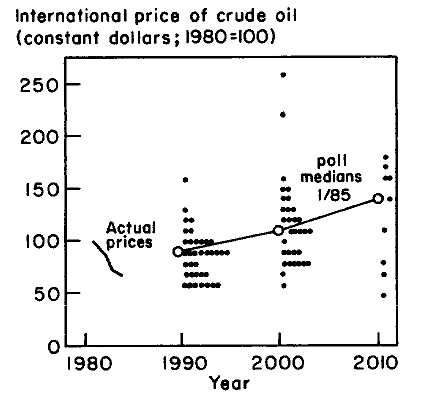
8.1. Price forecasts from 36 models, 1984. Source: Manne, Schratten-Holzer, and Svonronos (1985).
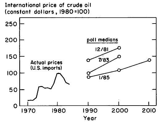
8.2. Price forecasts made in 1981, 1983, and 1985.
NINE
Wind Power in California A Case Study of Targeted Tax Subsidies
Alan J. Cox, Carl J. Blumstein, and Richard J. Gilbert
I. INTRODUCTION
The National Energy Act of 1978 and the California acts, AB 1558 and AB 3623, provided a 15% federal energy tax credit and a 25% California energy tax credit for investment in renewable energy sources. In addition to these tax incentives, California utilities, acting in compliance with the provisions of the Public Utility Regulatory Policies Act (PURPA), of-feted attractive rates for the purchase of power from independent electricity producers, further encouraging the development of wind systems.
Wind energy was one of the primary beneficiaries of these tax credits. The impact was greatest in California where a substantial wind industry emerged. In 1980 the California Energy Commission's (CEC's) short-term goal was to have 500 megawatts (MW) of wind-generated capacity on-line by 1987.1 In fact, there were 1,141 MW on-line by the end of 1985. The number of turbines installed rose from virtually none to over 13,000 by 1986, while energy production from wind grew from essentially zero to over 671 million kwh in 1985. By the end of 1987, there were 1,436 MW installed and 1,700 million kwh were produced from wind machines that year.
This remarkable development provides a good opportunity to examine the consequences of tax subsidies. In this chapter we look at these consequences from a number of perspectives, including those of wind investors, federal and California taxpayers, and California electricity ratepayers. We are interested in finding the costs and benefits of the program and in discovering whether the program could have been better
timed, by either limiting the amount of investment in wind turbines or altering the tax and price incentives. We undertake this analysis with the same benefit (and limitations) of hindsight that we employed in examining the Diablo Canyon nuclear project in Chapter 7. We also discuss the impact of the wind program on the direction in which wind technology has been developed. We use the term wind program to refer to the total package of tax incentives and energy payments available to builders of windmills.
The undiscounted economic cost of developing the wind industry in California, net of energy savings, could be as high as a billion dollars, with this cost distributed among electric utility customers and federal and California taxpayers. It is still unclear what costs and performance standards the wind industry will achieve.2 As a result we cannot be sure whether, for this public investment, a viable wind industry has been created. We do conclude, however, that the amount of investment in wind power in California has been excessive. Too much wind power has been developed at too great an expense, given actual and anticipated energy costs and requirements.
When Congress passed the National Energy Act in 1978, it hoped to achieve several objectives. These objectives included the enhancement of energy security after the 1973 oil embargo by reducing the share of imported oil used in U.S. energy production. Congress also wanted to encourage the development of cleaner, less environmentally damaging sources of energy. Despite these concerns, the 15% tax credit established for wind investments was passed almost as an afterthought, with little evidence that any attempt was made to estimate the cost and benefits of a wind subsidy program.3 The appropriate analysis should have included some examination of the optimal timing of subsidies if the goals listed above could not be met without such subsidies. Instead of providing such analyses, proponents of wind appealed to traditional arguments for "infant industry" subsidies. Not until about 1985, after the price of oil had collapsed, was there a substantial amount of analysis of the cost targets that windmills had to achieve in order to justify the program.4
The infant industry argument rests on the potential to exploit economies of scale by subsidizing early operations. An infant industry would
qualify for possible government support if the agents responsible for developing the technology and/or the product cannot appropriate the benefits of their work, as might be the case in basic research. These and other nonmarketable benefits that accrue to society in general are referred to as positive externalities.
Positive externalities are a crucial element in any justification of a subsidy to the introduction of a new technology. In the absence of positive externalities firms will attempt to introduce a new technology as soon as they expect that it can be profitably marketed. Therefore any subsidy directed at speeding up the introduction of the technology will merely reduce the net benefits to be derived from it. If there are externalities, then a subsidy might be justified because benefits will accrue to other firms and individuals.
In 1980 a company that undertook the task of developing an economical wind machine could not ensure that it would receive an adequate return on its investment in research. If the technology is easily imitated, with slight variations to avoid patent infringement, competition would limit the financial return from research and development. Alternatively, the government could undertake all the research and development work in wind and then transfer the technology to firms after it had been fully developed. However, the federal and California governments decided that the most appropriate way to overcome the roadblocks to wind power development was the establishment of generous tax credits and price guarantees for electricity sales.
Because tax credits were chosen as the instrument to spur the development of alternative energy sources, the capital to support that development had to come from private investors who could use the tax credits. With the interaction of the state and federal credits, along with the accelerated depreciation of the machines, most investors could recover about two-thirds of their investment through the reduction of their taxes in less than three years, even with no sales of electricity. If the turbine did perform as projected, the investor could expect to earn a high return (10-20%) from the investment. The large tax write-offs and the promises of wind energy electricity revenues attracted a huge amount of private capital and supported the rapid growth of the industry from 1980 until their expiration at the end of 1986.
There were also some deleterious effects of creating an industry with tax subsidies. The ease of raising private capital, whether through small private partnerships or much larger Wall Street brokerage house-sponsored partnerships, attracted wind farm developers and financial intermediaries with a wide variety of motives. Some manufacturers were more devoted to the sale of tax shelters than the development of a reliable wind turbine. Indeed, most investments failed to live up to their
promised levels of availability or production. Because the tax benefits were based on turbine capital cost rather than performance, it was easy for a developer to sell inferior machines at a hefty profit. A lack of any standardized performance rating system and the newness of the industry also contributed to developers being able to sell turbines with grossly exaggerated performance claims. In 1985 the California wind industry produced only 45% of the energy they projected it would produce (California Energy Commission, 1986b, p. 7).
The huge number of windmills that resulted from the wind program was clearly well above the number needed to develop the technology. But with tax credits in place and contracts to purchase electricity at guaranteed rates the government had little control on the number of windmill tax havens that were established. Once established, the wind incentives proved difficult to eliminate because alternative power providers had a strong incentive to keep the tax credits in place and the costs of the subsidy were spread over large numbers of taxpayers and electric utility customers.
In this chapter we first briefly describe the technology of producing electricity from wind. We then review government policies to encourage wind through its own research, through tax credits, and by mandating favorable rates for electricity purchased from wind generators. This leads to a brief discussion of the type of financial organization that most wind farms formed to maximize the private benefits of the government programs. We then undertake a detailed analysis of who paid the costs and who enjoyed the benefits from investments in two particular wind projects. The results there indicate that about 12% of the total costs of the wind projects were borne by the electric utility. The federal and California governments paid about 16% and 18%, respectively, in foregone tax revenue. In the next section we formally examine the infant industry argument by simulating the wind program. There we try to determine under what conditions, if any, launching an effort on the scale of the wind program would have made economic sense in 1980 or in subsequent years. We find that under the expectations for future prices of oil and gas, the economic losses from starting the wind program in 1980 were not huge. On the other hand, under the revised expectations brought about by the decline in world oil prices, the costs of continuing the program past 1983 should have been anticipated to be very large. The program should have been phased out at the end of 1983 as was called for under the original legislation.
II. WIND TECHNOLOGY
Figure 9.1 shows three basic designs of wind machines; downwind, upwind, and the vertical-axis Darrieus. Each has engineering advantages
and disadvantages. For instance, the downwind machines do not require any controls to keep them pointed into the wind (yaw control), but they lose energy due to the tower's shielding effect, which also results in uneven strain on the rotors. Darrieus windmills, the object of considerable federal research efforts, incorporate the gearbox and generator on the ground. This configuration allows for easier servicing and reduces the amount of structure that would otherwise be required to hold this machinery aloft. In addition, the Darrieus windmill does not have to be pointed into the wind either, thus eliminating the need for yaw control.
Machines are also classified as small (rotor diameter 5 meters or less), intermediate (5-30 meters), and large (30 meters or more). Small to intermediate windmills can be made of relatively simple, off-the-shelf components. Large windmills, however, require more elaborate controls and very heavy structures to prevent damage in high-wind situations. A large part of the research effort in large-scale wind turbines has been in developing the control components and in paring down the size of the structures to reduce cost while at the same time maintaining a reasonable level of reliability.
Most government research effort in the 1970s focused on large machines. Possibly the best result of tax-induced private investment in wind is the diversification it provided in development. Although there has been no commercial spinoff from the government's large windmill effort, private investment has resulted in impressive improvements in the intermediate-scale technology. Reasons for this divergence between the government's research and private development are discussed further below. It may yet turn out that the large-scale wind systems will provide the lower-cost technology.
Large turbines typically have generators above 1 MW, intermediate-sized between 50 and 250 kW, and small turbines are in the range of 1 to 10 kW. The appropriate size of generator for a particular size of rotor depends on wind variability and average wind speed. Figure 9.2 shows output versus wind speed for a hypothetical wind turbine. Below the cut-in speed, the machine cannot operate; above this speed output rises rapidly until the rated speed is reached. Above the rated wind speed, output is constant until the wind reaches the cut-out speed. At that point the machine is turned off to protect it from damage that might result from the stresses of high winds.
The choice of rated speed involves a trade-off between the extra output that can be obtained at higher rated speeds and the extra cost of a larger generator. These trade-offs will be modified for different locations by the distribution of wind speeds. The trade-off is made more complicated by the fact that a windmill operates more efficiently if it rotates faster at higher wind speeds. However, conventional alternating current generators can operate only at a single fixed speed. Requiring rotors to
turn at a fixed speed reduces system efficiency at most wind speeds. The energy in wind increases with the cube of its velocity, but the varying efficiency of the turbines at different wind speeds due to the fixed-rotation constraint results in less than cubic increase in output with wind speeds.5 Efficiencies are improved by some turbine manufacturers by having two generators, the higher rated of which (in terms of kilowatts) is substituted for the smaller generator as wind speeds increase. Windmills can also be geared at varying ratios, allowing discrete jumps in turbine rotation as wind speed increases.
Because actual wind speed is lower than the rated speed much of the time, the effective capacity of a wind generator is lower than its rated or "nameplate" capacity. The ratio of average output to nameplate capacity (the capacity factor) depends on the wind speed distribution for the site, the curve of output vs. wind speed for the machine and its availability. A typical machine at a good site would have a capacity factor of from 15% to 30% if it operated perfectly and its maintenance could be scheduled when average wind speeds were low.
The intermediate-sized turbines currently prevalent in California have been located in wind parks in which large numbers of wind turbines are clustered. This arrangement offers economies in the construction of roads and tower foundations; in the use of substations, transmission lines, and control facilities; and in maintenance. The clustering of turbines on wind farms does result in problems of interference among windmills, creating variation in power production.
These interactions and, more important, the variability of wind speeds result in wind being a stochastic source of supply. There is already an extensive literature on estimating the value of randomly available electricity supply.6 The basic concept is that these systems should be credited with the increased reliability that they provide the system. In essence, they are credited with the expected value of the capacity that they produce at a particular, critical time. This is analogous to the treatment of dispatchable power in that there is always some probability that a power plant will not be available when required.
The appropriate credit for wind is something that will change as our understanding of the systems improves. Wind is generally more available in the summer months when California's demand for electricity is greater. On the other hand, peak daily wind output misses the system
daily peak demand by about eight hours (Smith, 1987, p. 178, and see Chapter 6 of this volume).
Despite this particular phenomenon, wind generation clearly should be given some capacity credit. Smith (1987) estimates a capacity credit equal to 13% of the nameplate capacity of the wind turbines in the Alta-mont Pass. Other areas of the state may provide superior load-matching capabilities.
III. GOVERNMENT POLICIES SUPPORTING THE DEVELOPMENT OF WIND ENERGY
Research and Development
Before the Arab oil embargo there was little government support for the development of wind energy. After the embargo, fairly substantial expenditures were made by the Department of Energy (DOE) and its predecessor agencies. Total expenditures for wind energy research and development in the fiscal years from 1973-1985 were $391 million. These expenditures were small initially but grew rapidly to a peak of $63.4 million in FY 1980 during the Carter administration. They fell steeply during the Reagan administration; expenditures in FY 1985 were only $29.1 million.
Table 9.1 shows the DOE funding by category. The centerpiece of DOE's program has been the development of very large wind turbines. The development efforts have progressed through a series of prototypes and are now focused on producing machines that will have a capacity in excess of 3 MW. These machines are intended to be suitable for commercial use in the 1990s, producing electricity at 4¢/kWh (1985 dollars). Direct expenditures for design and construction in this development effort have consumed approximately a third of DOE's wind-energy budget.7 In addition to the direct expenditures, work that was primarily for the support of large-turbine development consumed a significant fraction of the funds in the "generic" category.
Results from the large-turbine development program have not been very encouraging to date. Only a few large machines have been built, and none of these machines is operating reliably. Among companies that were experimenting with large wind turbines, several have dropped out of the industry or severely cut back their involvement.8 Although DOE remains officially optimistic, development seems to have shifted
decisively to the intermediate-scale machines. As discussed below, this shift may have arisen from the desire to spread an investor's performance risk over several machines rather than a single large machine and cannot be taken as compelling evidence of the superiority of intermediate-scale technology.
The productivity of other research and development expenditures is harder to assess. Darrieus turbines received substantial support. Intermediate-scale versions of these machines were deployed in significant numbers by private developers. In addition, many of the engineers currently working in the field got their initial experience working on government contracts. Needed engineering data and techniques were developed with government support. In sum, however, given the expenditure of $391 million, results from the DOE wind energy program have been modest.
Tax and Financial Assistance to Wind Generators9
Federal Programs—Tax Credits and Depreciation Allowances. The Energy Tax Act of 1978 (PL 95-618) established a business investment tax credit for certain energy properties including wind turbines. The tax credits were 15% of the amount invested and expired on December 31, 1985. This tax credit was in addition to the 10% investment tax credit (ITC) in effect over the same period.
Wind investments also benefitted from rapid depreciation under the accelerated cost recovery system (ACRS) established in 1981 as part of the Economic Recovery Act. The ACRS provided for a five-year depreciation of wind turbines. Although ACRS and the ITC also applied to most other investments, it had stronger incentive effects on capital-intensive projects such as wind. Furthermore, utilities were specifically excluded from using ACRS and the energy tax credit.
Federal Programs—Technical Assistance and Loans. Under the Wind Energy Systems Act of 1980, DOE had $100 million authorized in 1980 for cooperative agreements, outright grants (not exceeding 50% of the cost of the wind system), and subsidized loans. Additional federal support was available from the Small Business Administration in the form of loans and loan guarantees. Other programs of the federal government could be used by particular categories of potential purchasers of wind systems for their own use, including cooperatives, farmers, nonprofit corporations, public agencies, and homeowners. Neither the federal government's research program nor its technical assistance and loans are included in the cost/benefit analysis in this chapter.
California Programs. The most important of the California programs that applied to wind farm developers was a 25% energy investment tax credit. This credit was reduced to 15% on January 1, 1986 and expired completely on December 31, 1986. Accelerated depreciation was also available, although not on terms as favorable as ACRS.
The net effect of these tax advantages for an investor depended on the investor's marginal tax rate, interactions between state and federal taxes, and the financial arrangements involved. Typically, between 60 and 80% of the gross investment was returned to the investor as a consequence of these tax advantages. In many cases, the total cost of an investment could be recovered in three to five years even if no electricity was produced (provided that the Internal Revenue Service did not view nonproduction as a reason to "recapture" the tax credits).
Public Utility Regulatory Policies Act
Tax advantages alone would not have stimulated significant development of wind projects without other government actions that were taken to make a market for the energy produced. These actions included passage of PURPA by the Congress in 1978 and implementation of the act in California by the California Public Utility Commission (CPUC). PURPA required utilities to purchase electricity from independent power producers at prices corresponding to avoided costs. Interpretation of the language of the act has caused considerable dispute over the extent to which avoided cost should reflect short-run or long-run marginal cost. Although this controversy is still simmering, it is sufficient for the purposes of this chapter to know that the prices offered by utilities under the CPUC's jurisdiction were high enough to provide encouragement for wind developers; peak rates paid to some producers by PG&E were 24 cents/kWh during one period in 1984 (Smith, 1987, p. 149).
In California contracts were established between independent power producers and electric utilities by the mechanism of Standard Offers. Under state regulations, public utilities in California must buy power from independent producers under the terms established by the CPUC. The last and most attractive of those contracts, Standard Offer 4 (since suspended), set off a stampede of potential power producers signing contracts with utilities. One option under this contract was particularly attractive to those attempting to establish wind farms. This option locked in for a period of 10 years an escalating series of prices for energy and capacity delivered to the utility's grid. The price was based on forecasts of the utility's marginal energy costs. This reduced uncertainty about prices, making the raising of capital for wind farms easier. With the decline in oil and gas prices in 1986, it became apparent that the long-term standard offers were much higher than expected avoided
costs and the CPUC indefinitely suspended these offers. However, independent electricity producers who already had signed contracts to sell power under these terms and with the required approvals were not affected.l0
IV. THE EFFECT OF THE WIND ENERGY PROGRAMS ON CALIFORNIA
Installed Capacity
California has become the world center of wind energy development for several reasons. These include the 25% state tax credit, avoided-cost rates favorable to alternative energy producers, some good wind locations, and a relatively large number of wealthy individuals with sufficient income to take advantage of the tax incentives. Of all electricity produced from wind in the world during 1985, 87% was produced in California. According to estimates by the CEC and reports from California utilities as shown in Table 9.2, the number of machines installed grew from 144 at the end of 1981 to over 13,000 at the end of 1985. During this period, rated capacity grew from 7 MW to 1,141 MW; by the end of 1987 total cumulative investment was in excess of $2 billion in nominal dollars.
The largest site for wind farm development in terms of power produced is the Altamont Pass area, which contains about 60% of all machines installed in California. Other important sites for development are San Gorgonio Pass (23% of installed machines) and Tehachapi Pass (21%). Figure 9.3 shows the locations of these sites.
Technological Development
The wind industry has made substantial improvements in the quality of intermediate-sized windmills since 1981 when the first machines were sold. Reliability has improved significantly, resulting in higher capacity factors.11 Capacity factors for 1985 averaged 17% at Altamont, 18.4% in San Gorgonio, and 13.8% in Tehachapi (California Energy Commission, 1988, pp. 117-119). Although these are well below the 25 to 35% predicted by wind proponents, they represent a significant improvement over the early experience.
In addition, the cost of wind turbines has fallen over time. The average price of a wind turbine in 1981 was $3,984 (in 1986 dollars) per rated kilowatt. By 1985 this figure had dropped to $1,900 (California Energy Commission, 1986a, p. 17) and may now be as low as $1,100 (Smith, 1987). The ultimately achievable cost for windmills is still not clear, and estimates of the possible costs vary. What projections are published come with little substantiation. A low estimate is provided in a report to the CEC (California Energy Commission, 1988), which forecasts $600/kW. Smith (1987) suggests that $750/kW may be attainable while the Office of Technology Assessment (1985) provides a range of $900-$1,200/kW for the 1990s.
The strong tax incentives to private investment in wind systems provided an alternative approach to the development of wind from that of the government. One of the most striking differences between government-sponsored wind research and the strategy adopted by private developers has been the size of the wind turbines. It was originally believed that the most efficient way to extract electrical energy from the wind was with large, megawatt-scale machines. The technical complexity and early difficulties with large windmills resulted in the refusal of the manufacturers to guarantee the performance of their machines.12 Without assurances from the manufacturer as to the turbines' performance, investors were unwilling to underwrite a large turbine wind farm.
The lump-sum costs of wind turbines was another major influence in the popularity of the intermediate turbines over the large turbines. At a cost of $5 million and more for a large turbine, the risks to the investor, in the absence of a proven performance record, were too great. (This cost compares with between $150,000 to $300,000 for an intermediate-sized turbine.) Instead of a few large turbines, windmill manufacturers (who had to provide performance guarantees) chose to produce and sell many intermediate-sized turbines, thereby spreading the performance risk over many more machines and enabling them to lower costs through higher production levels. It was also easier to isolate and identify turbine problems with a greater number of machines to compare and analyze.
The fact that intermediate-sized windmills were used in private investments does not prove that they represent the best solution to extracting energy from wind. All that can be said is that they were the most readily available technology to take advantage of high electricity prices and tax incentives. As we show in this paper, the intermediate-scale technology has not provided a cost-effective source for electricity. If wind ever does become commercially viable, it may yet be large windmills that will provide the most economic use of this resource.
The nature of the inducements to the wind industry also resulted in a wide variety in the design of intermediate-scale windmills. However, there were some clearly economically wasteful results of the capital-biased nature of the tax incentives that manifested themselves in the wind program and limited the variety of designs. As we have stated, the incentives allowed the cost of an investment to be recouped in three or four years even with no significant output. Such a scheme is bound to result in some systems being built with little prospect of producing large amounts of electricity or of providing any information to further improve the technology.
A more subtle waste is due to the tax-induced preference for higher up-front cost and lower operations and maintenance costs. The tax benefits allow investors to reduce the net cost of the initial investment, whereas yearly overhead and maintenance expenses continued to be treated in the same way as any other investment might be.
This bias might go some way to explaining the popularity of Danish wind machines. These machines were certified (in a program of the Danish government) to withstand the stronger average winds off the North Sea. Not only was maintenance lower in these machines, but they had a reputation for quality construction and superior reliability in an industry where reliability is one of the major unknowns and consequently of great importance to general partners and investors. Failure of a turbine to remain in service for five years after a tax credit was taken would result in serious potential financial consequences to investors in the form of a tax credit recapture and other penalties.
Financial Organizations of the Wind Industry
Two forms of ownership arrangements of wind turbines are prevalent in the industry: limited partnerships and direct ownership by individuals or small general partnerships. Limited partnerships are the dominant form of organization; direct ownership is a relatively recent innovation. Often the limited partnerships have direct or indirect links with a wind turbine manufacturer. A common practice is for the manufacturer to incorporate a wholly owned subsidiary in California. A limited partnership is organized by the subsidiary with the subsidiary as managing general partner. The managing partner then sells limited partnership interests to investors. The proceeds from these sales (less commissions and other fees) are then applied to the purchase of wind turbines from the manufacturer who initiated the whole process. In addition to the proceeds from the sale of partnership interests, the manufacturer may receive a note from the partnership for a portion of the wind turbine sale price (e.g., if the sale price were $170,000, the partnership would pay $100,000 in cash and would give the manufacturer a note for $70,000).
This type of arrangement has some significant advantages for investors. First, a limited partnership does not pay income tax; the profits and losses flow through directly to the partners. Thus the limited partners receive the tax credits and the losses that result from depreciation (subject to limitations in the tax code). Second, a limited partnership provides limited liability; if the partnership defaults on its loan, the limited partners are not liable for this obligation. The note that the manufacturer takes back is usually nonrecourse (i.e., unsecured by any assets other than windmills) with terms of 10-20 years. Because the note is included in the basis of the investment, it increases the tax credit available without increasing the necessary investment.
The limited partnership form of organization does have some disadvantages. The commissions and other fees associated with organizing and offering the limited partnership units are not eligible for tax credits. Losses are limited to the amount at risk (i.e., the amount invested net of any income received). Finally, although the investor is not liable for the partnership's notes to the manufacturer, some of his tax credits can be recaptured by the government if the partnership defaults.
In a direct ownership arrangement, a wind turbine is purchased outright by an individual or small general partnership. The financing, if any, is recourse to the individuals involved (i.e., the lender has a claim on other assets of the borrower in addition to the wind turbine). The advantages of this arrangement are that the entire purchase price is eligible for the tax credits, deductions for losses may be greater because of the higher amount at risk, and the risk of recapture of tax credit is reduced because no nonrecourse financing is involved. The disadvantage is, of course, that the investor has 100% of the purchase price at risk (as opposed to approximately 60% in a limited partnership) and thus his losses may be greater if the wind turbine fails to perform. Also, default on his recourse debt may lead to (property) losses other than his wind investments.
The Detailed Economics of Wind Projects
In this section we quantify the costs incurred and the benefits gained by different parties in two wind farm projects. Before doing so it is instructive to look at the impact of the federal and state tax credits on the private costs of wind-generated electricity. Table 9.3 shows the amount by which the tax credits alone bring the private costs of electricity below the social costs.13 (Depreciation and operating costs are handled exactly the same way for both cost calculations.) The results indicate that, depending
upon the capital cost assumptions, the private cost is between 40% and 55% of the total social cost.
In order to identify all the costs and benefits to the participants of a wind project, we analyzed two projects. The projects being modeled are organized as a limited partnership. The parties included in our consideration are the investors in the wind farm (the limited partners), the government of California, the federal government, and the ratepayers of the utility that is buying the wind farm's electricity. In addition, the project is also evaluated from the point of view of the economy as a whole. The net economic benefit of a wind project is the cost of the electricity displaced by wind minus the economic costs of the wind project. (Economic costs do not include such transfer payments as property taxes.) The benefits to the two levels of government are merely the increase in the tax revenue due to the wind project net of tax revenue that would have been earned on alternative projects. Profits are the change in the after-tax positions of the investors in this partnership, net of after-tax profits that could have been earned on other investments. The costs of a wind project to the utility ratepayers is the amount paid by the utility to the wind farm operators minus the reduced expenditures by the utility to produce electricity. The amount paid for the electricity will, for the first 10 years of the project, be determined by projections made under Standard Offer 4 contracts. As noted above, these contracts called for high payments to the windmill-owner for electricity purchased by the utility. The payments were so high that purchasing electricity imposed a cost on the utility, not a saving. All costs and benefits of the project are discounted back to 1985 at 10%. For the private investors, this is an after-tax discount rate. Except where otherwise noted, all costs and benefits are taken from the partnership offerings.
The first project being modeled here, FloWind Partners 1984, is one that was constructed during the latter part of 1984 and early 1985 and is located in the Tehachapi Mountains. According to the prospectus, the general partners expected the price of electricity sold to Southern California Edison (SCE) to reach 12.8¢/kWh (nominal) by 1994 from 6.6¢ in 1985. About one-sixth of these payments were for capacity. We use these price projections through 1994 (correcting for their inflation assumptions), after which the price is held constant in real terms. The base case also utilizes the pre-1987 maximum marginal federal tax rate of 50%. We do not take into account any at-risk provisions of the tax code.
The construction cost of the project, as described in the prospectus, is $36.6 million. Another $4 million was required to cover organizing costs and working capital requirements, giving a total cost of about $41 million. Of this, $25 million was equity raised from the limited partners with the rest coming as a loan from the FloWind Corporation. The
project had an expected total output of 45,600 MWh per year generated from wind turbines that are rated at about a total of 22,000 kW. The construction costs give a cost per kilowatt of about $1,700. Under these base case assumptions, the equity portion of the investment would be fully recovered after 3.5 years even if no electricity is produced.
Columns I and 2 of Table 9.4 show some of our other results for the FloWind project. The largest contributor to the project (net of benefits) is SCE, which will pay almost $35 million for the power projected to be produced by FloWind. The present value of avoided costs in that service area, under our base case assumptions (see Table 7.3) is about 5.6¢/kWh. That means that about $8.5 million of the $26.7 million will be paid by SCE to FloWind over and above the cost to the utility of producing that electricity itself. The largest government contribution made to covering the cost of the project ($8.4 million in 1985 dollars) is that of California. The federal government's total contribution through the additional 15% tax credit (partly offset by the decreased state tax deductions due to California's tax credit) is $7.44 million. The net present value of the project to the limited partners is almost $1.75 million, not huge considering the riskiness of the investment. The present value of the economic cost of the wind farm, including operating and maintenance, is over $48 million.
The public costs do not include the ITC and the ACRS because these can be taken for most other investments and therefore do not result in a net economic cost to the governments. However, the ACRS cannot be taken by electric utilities. To the extent to which wind investment displaces conventional investment by electric utilities, the cost of wind to the governments is understated in Table 9.4.
The third and fourth columns of Table 9.4 present the same figures for an investment as a partner in a single machine of the Zond program. This program, which was scheduled to come on line in 1986, sold individual turbines in a project in the Tehachapi Mountains for $175,000 or a cost of about $1,871/kW when capacity is measured at maximum rated wind speed.
The California government has a lost revenue of over $38,000 for each turbine in this project. The federal government's contribution is $36,000. But SCE makes the largest contribution. Of the present value of SCE's expected per-windmill payments of $144,000, about $45,000 will be above its costs to produce an equivalent amount of electricity. The full economic cost of a windmill in this project is $219,000.
The larger per-kilowatthour profit for the Zond Painted Hills windmill is due to the much higher capacity factor that the Zond partnership forecasts in its prospectus (30% as opposed to 23%) and the slightly higher capital cost, allowing for a greater deduction of the investment
tax credit. Both projects show an average variable cost of about 2.3¢/ kWh. These costs include operations and maintenance, management fees, land rentals, and insurance but exclude property taxes14 and are in general agreement with those found in Smith (1987).
Table 9.5 illustrates the sensitivity of the financial performance of the FloWind project to the underlying assumptions. The first two columns of the table indicate the net benefits to the partners if, after the 1995 expiration of the partnership's electricity purchase contract, the price paid for electricity is close to that predicted by the CEC. The other two columns indicate the results if the price of electricity after 1995 is based on the base case assumptions used to evaluate the Diablo Canyon nuclear project in Chapter 7. These numbers indicate that the total overpayment by SCE will likely be on the order of $6.7 million when discounted back to 1985.
The calculations undertaken for these wind projects indicate the importance of the tax credits and the high expected payments to the wind farms for the electricity produced. Of these, the tax credits clearly had the largest impact on the expected profitability of these projects. They represented about one third of the total discounted costs of the ventures. SCE ratepayers would provide another 18% of the total cost if the difference between the value of the electricity displaced by wind and the price paid for that electricity persists. In addition, a downward shift in any of the very favorable projections included in the prospectuses would result in serious losses to the investors.
Optimal Timing of a Wind Program
Expenditures on commercial wind systems in California have totaled over $2 billion, and in this section we discuss the net economic benefits of these expenditures. In particular, we are interested in the timing of wind energy investments and when, if ever, it would have been economically rational to enter into such a program. To undertake this analysis it is necessary to make predictions about the cost of wind energy in the future. These predictions are then compared with the estimates of the value of the energy and capital that is displaced by wind. To measure the efficacy of the wind program, we also have to make some assumptions about the behavior of potential investors in the event that there were neither tax incentives nor high purchase rates. We can use these assumptions about behavior to evaluate the efficacy of alternative programs.
Before we estimate the costs of a wind program, it will be helpful if we have some idea of the sort of cost reductions that would have to be
achieved for wind to be a competitive technology. In Table 9.6 we show the maximum costs of wind turbines necessary for wind to compete with fossil-fuel-fired gas turbines. The capacity credit for wind is assumed to be 0.5¢ kWh, and the heat rate for the plants displaced by wind is assumed to be 11,300 or 10,300 Btu/kWh, in keeping with our assumptions from the Diablo Canyon review. The variable cost of the wind turbines are assumed to be 2.5¢/kWh. The first column of Table 9.6 shows different possible costs of the wind turbine in $/kW. Column 2 shows the resulting average total cost of wind-generated electricity. Column 3 shows the cost of oil, in dollars per barrel, that wind turbines could compete against at the prices shown in column 1. For example, if the level-ized cost of oil is $30/barrel, and the heat rate of the oil-burning plants displaced by wind averages 11,300 Btu/kWh, then the capital cost of wind energy would have to be less that $700/kW for wind to be competitive with oil-fired capacity. To evaluate the wind program we first estimate the costs and benefits of the program through the end of 1985. We assume that at the end of 1985 all investment tax credits are terminated and that no new wind farms are built. Windmills that have already been built continue to produce electricity.
Electricity is sold to California utilities at prices that are established by contract when the windmill comes on-line. The prices established in these contracts are assumed to be based on ten-year forecasts of the cost of electricity. The projections used are for a 3%/year increase of the value of electricity from the date that the wind project comes on-line.15 All costs and benefits are discounted back to 1980, the assumed first year of the program. The costs of installed wind turbines are those found in Smith (1987).
Table 9.7 indicates that the present value of the capital and operating costs of all windmills built through 1985 is $1.8 billion, and the fuel and capacity savings are $1.1 billion. The negative net benefits of $463 million were paid for by $373 million in tax subsidies and $152 million in payments by electric utilities over and above their own costs of producing electricity. (Recall that these are all present values discounted back to 1980.)16
But some of the windmills that were built while the tax program was in effect would have been built anyway, although possibly not very many.
Also, the infant industry argument predicts that more windmills would have been built sooner once the program was over, because the industry would have been brought down the learning curve by the program. To measure the net effect of the wind program, we have to make some assumptions about the manner in which investment in wind would have taken place in its absence. We also have to make some assumptions about the effect of wind investment in driving down the cost of windmills.
A fairly simple model of investment in wind was created to examine this question. The total capacity of installed windmills for any given year is described by an investment schedule the first five years of which is made up of the investment figures presented in Table 9.2. For later years the investment consists of a logistic function that is parameterized to fit the last year of the wind program's investment history. The cost of wind systems is a decreasing function of the installed capacity of windmills.
None of these relationships are statistically estimated because there are not many years of data. Instead we have calibrated the model to fit the data that we have available. Once the results presented below were generated some sensitivity runs were undertaken by changing the parameters of the model. None of the conclusions were appreciably altered. In our simulations of the wind program from 1980 we employ, for oil prices, base-case expectations of a 3% real increase from the observed price from 1980. We also present results under the assumption that a 1% increase in oil prices was expected. Heat rates for the fossil fuel plants that wind might displace are based upon the same average heat rate that is presumed to prevail in the Diablo Canyon study; 11,300 Btu/kWh.17 In all cases the average capacity factor ultimately achieved by windmills is 25%. The average operating cost of the windmills is assumed to be 2.5¢/kWh.18
We first used this model to predict the optimal timing of a wind program, given the expectations for oil price increases and assuming that yearly investment in wind is characterized by our logistic function. The optimal time of a wind program is characterized as the year of initial wind development that maximizes the discounted net benefits of the wind program.19 It is the year in which a profit-maximizing firm that had a monopoly on wind production would initiate its own wind program. This rule is also the appropriate one that the government should employ, optimizing the expenditure of funds so that all the benefits (in-
cluding the external benefits) exceed the costs by the greatest amount. Searching for the optimal time to begin the program was undertaken merely by shifting the investment schedule described above from year to year and comparing the net present values of the program started in different years.
Table 9.8 presents estimates of the net benefits of the wind program under different scenarios. The first row of results assumes that oil prices rise at the 3% rate from their 1980 levels; the second row shows the results of an expected 1% real increase in prices. Columns 1 and 2 show the results if the cost of wind turbines falls to $900/kW; columns 3 and 4 contain results using the $700/kW ultimately achievable cost. Columns 1 and 3 show the result of starting the program in the year that resulted in the highest net present value of the program, whereas columns 2 and 4 show the result of starting the program in 1980.
Turning first to the 3% real increase expectations: For the $900 windmill capacity cost, our results indicate that the optimal time to have started the program was in 1984. In that case the present value of the program would have been $667 million. Starting the program in 1980 would have resulted in net benefits of $561 million, had prices risen as forecasted. The loss from starting the program early was $106 million. Under the lower windmill price scenario, the loss to starting the program in 1980 instead of the optimal year was only $40 million.
Under the assumption of a 1% real increase in oil prices there is no time before the year 2000 that it would have made economic sense to start the wind program. The losses due to starting the program in 1980 are $406 million for the $900 cost scenario and $139 million for the lower-cost scenario. These losses would have had to be recovered from either tax credits or overpayment for wind-generated electricity.
The results in Table 9.8 indicate that only under very favorable cost and price scenarios was it worthwhile to proceed in 1980 with a wind program of the scale that eventually transpired. Although there is still some uncertainty about the costs that windmills will achieve, it is now clear that the sort of high-oil-price scenarios that would have justified a large-scale wind program are no longer likely to be borne out. Our re-suits indicate that the program could have been profitably postponed (when profits include only the measurable costs and benefits of the program). Had it been postponed, additional information on the likely price path of oil would have been available. On the other hand, losses due to starting the program two years early were not great had there been a reasonable expectation that wind machines were going to cost $700/ kW and oil prices were going to continue to rise at a very high real rate.
However, it was clear by 1983 that prices for oil were going to be well below the lower of the trajectories assumed for Table 9.8. Given what
was known about oil prices in 1983 and given the experience gained in producing electricity from wind, it seems reasonable to ask whether it was appropriate to continue the program after the end of 1983. That year is an appropriate date upon which to base a review because the California Tax credits were scheduled to expire on December 31 and the CEC undertook such a review of all solar, wind, and conservation credits (California Energy Commission, 1983).20 The legislature eventually extended the credits beyond their initial sunset date.
To determine whether it was appropriate to continue the program, we reran our simulations retaining the reductions in the cost of windmills that had been achieved through 1983. Here we are undertaking essentially the same analysis that we did for the Diablo Canyon study. We are ignoring previous expenses, treating them as sunk, unrecoverable cost. Also, we assume a 1% real increase in the cost of oil from its 1985 level.21
The previous investment results in the achievement of an average cost of windmills in 1984 of $1,400. Even if the ultimately achievable cost was expected to be $700/kW, continuing the program to the end of 1985 resulted in a net present value of —$560 million. The investment tax credits absorbed about $278 million of this expenditure. Despite these huge losses, no wind industry could expect to be established. We can see this by looking at the results presented on Table 9.6 which shows that, at the price of oil prevailing in 1985 (see footnote 21), windmills would have to cost less than the target $700/kW.
If we ignore the externality arguments necessary to the infant industry justification of the program, proceeding with the wind program can only be justified if the ultimately achievable cost is so low that the returns in later years in reduced energy costs will offset the high costs of the initial development of the wind machine. We can use our model to determine the per-kilowatt cost that would have to have been thought achievable to raise the net present value of the wind program to zero. That price would have to have been $550/kW. This figure is below any of the estimates found in the literature for intermediate-scale wind turbines.
In summary, these simulations were undertaken under fairly optimistic assumptions for the ultimately achievable cost of wind machines, the
rate at which these costs would be achieved, and the windmills' capacity factor. Oil price forecasts were also high. If the predictions for wind technology were reliable, then proceeding with a wind program in the first half of the decade would have achieved the highest present value for the program. Proceeding with the wind program in 1980 resulted in relatively small decreases in the present value of the program.
On the other hand, the costs of proceeding with the wind program beyond the end of 1983 have been high. Taxpayers and electric utility customers in California could have saved at least half a billion dollars had the program been terminated then. In fact, the total saving would probably have been greater because it is unlikely that wind will achieve a cost of $700/kW.
It is important when considering these estimates of the losses of the wind program to remember that they do not include any of the research costs listed in Table 9.1. These amounted to almost $400 million by 1985. Nor do they include the cost of other funding, through grants and loan guarantees, available from the federal government and described above. The allocation in 1980 alone for these programs was $100 million.
V. CONCLUSIONS
The scale of the development of the wind industry was an almost unanticipated result of various tax expenditure programs and the regulatory changes of PURPA. The cost of the program, net of any fuel savings, will be about half a billion dollars when discounted back to 1980. The largest part of these costs was borne by federal and California taxpayers with the electric utility ratepayers also contributing large amounts. These costs do not include expenditures on research or technical assistance.
In 1980, it was not unreasonable to undertake a wind program given the prevailing expectations of future energy prices. However, it would have been better to delay the wind program in California by at least two more years. By that time more information would have been available on the ultimately achievable costs and on the likely trajectory of oil prices.
As expectations of future energy prices changed to reflect lower then-current prices, it was much less easy to justify the continuation of the program after 1983. By that time an annual 3% rate of increase in the price of oil from real levels that prevailed in 1980 was not a reasonable scenario. The cost of continuing the program beyond that point is at least half a billion dollars, discounted back to 1983. This cost is based on a continuous 1% annual increase in oil prices from 1983. In fact oil prices have dropped another 35% since then.
These expenditures have not led to the development of a wind power industry that is likely to be economically viable in the next 10 years, given recent forecasts of energy prices. Tax subsidies were so large and CPUC-mandated prices were so high that investments could be made in wind farms with little concern for maintaining the long-term viability of a firm in the industry.
These conclusions tend to underline problems that arise with subsidies of the sort that were used in the development of the wind industry. In the absence of major externalities, an infant industry or new technology that is likely to be viable in the long run will not need subsidies. Infant industries or new technologies that cannot survive without massive subsidies will likely fail anyway. The extent to which subsidies are used to encourage new industries or technologies should be limited.
The amount of wind power capacity that is currently installed in California is about three times the original goal set by the CEC. Had this goal been maintained and had other, performance-based, incentives been provided, the wind program would certainly have cost less. It may also have been more successful at achieving the technological targets that were expected to be achieved. Several performance-based incentives could have been used. For instance, the government could have auctioned the right to have access to price supports which would then only be available upon certain performance goals being met.
This study also shows the cost of not terminating a program after circumstances are altered. No special legislation was required to kill the tax credits. In fact, the opposite was true; the original California legislation had a provision that eliminated the credits at the end of 1983. In effect, the nonsunk-costs arguments of Chapter 7 are reversed to some extent here. Expenditures made in subsidizing wind through 1983 should have been ignored in any evaluations of future expenditures. It is inappropriate to make further expenditures just because so much money has already been spent.
REFERENCES
California Energy Commission (1980a). "Renewables and Alternative Technologies Synopsis, Staff Draft," P500-80-012, Sacramento.
California Energy Commission (1980b). Solar/Wind Programs, Final Environmental Impact Report . P700-80-005.
California Energy Commission (1983). "California's Solar, Wind, and Conservation Tax Credits, Draft Report." Tax Credit Committee, P103-83-001.
California Energy Commission (1986a). Results From the Wind Project Performance Reporting System, 1985 Annual Report , P500-86-013.
California Energy Commission (1986b). Solar and Wind Technology Tax Incentive Impact Analysis , Report Prepared by Polydyne, Inc. P500-86-010.
California Energy Commission (1988). Forecasts of Annual Capacities of the Supply of Electricity Likely to be Available from Quailing Facilities Not Subject to CEC Jurisdiction , Prepared by Regional Economic Research, Inc.
Energy Information Administration (1987). Monthly Energy Review , October. DOE/EIA-0035(87/10).
EPRI Journal (1980). "Going With the Wind," Vol. 5, No. 2, March, pp. 6-18.
EPRI Journal (1984). "Wind Power: A Question of Scale," Vol. 9, No. 4, May, pp. 6-16.
Hirsh, E., L. Briefly, and V. Schwent (1981). "A Guide to Financial Assistance for Wind Energy," Sacramento: California Energy Commission.
Kahn, E. (1979). "Wind and Solar With Conventional Technology," Annual Review of Energy , Vol. 4, pp. 313-352, Palo Alto, Calif.: Annual Reviews, Inc.
Katzman, M. T. (1984). Solar and Wind Energy An Economic Evaluation of Current and Future Technologies . Rowman and Allanheld.
Merriam, M. F. (1986). "Wind Electricity for California: Costs and Benefits," Universitywide Energy Research Group Working Paper No. UER-164, Berkeley: University of California.
Office of Technology Assessment (1985). New Electric Power Technologies: Problems and Prospects for the 1990s , Washington, D.C.: OTA-E-246.
Smith, D. R. (1987). "The Wind Farms of the Altamont Pass Area," Annual Review of Energy , Vol. 12, pp. 145-183, Palo Alto, Calif: Annual Reviews, Inc.
Solar Energy Research Institute (1981). A New Prosperity, Building a Sustainable Future, The SERI Solar/Conservation Study. Andover, Mass.: Brick House Publishing.
Tabors, R. D., S. Finger, and A. J. Cox (1981). "Economic Operation of a Distributed Power System Within an Electric Utility," IEEE Transactions on Power Apparatus and Systems , Vol. PAS—100. No. 9.
Van Kuiken, J. C. (1980). "Reliability, Energy, and Cost Effects of Wind-Powered Generation Integrated With a Conventional Generating System," Argonne, Ill.: Argonne National Laboratory, ANL/AA-17.
|
TABLE 9.1 |
||
|
Expenditure |
% of Total |
|
|
Intermediate and Large Turbines |
202.1 |
51.7 |
|
Small Turbines |
60.0 |
15.3 |
|
Darrieus Turbines |
22.3 |
5.7 |
|
Generic a |
106.8 |
27.3 |
|
NOTE: Includes policy studies, wind resource assessments and fundamental engineering studies. |
||
|
TABLE 9.2 |
|||||
|
Before |
1982 |
1983 |
1984 |
1985 |
|
|
Cumulative Number of Turbines |
144 |
1,300 |
3,800 |
8,100 |
13,500 |
|
Investment/Year ($ In Millions) |
21 |
139 |
326 |
680 |
1,100 |
|
Installed Capacity (MW) |
7 |
71 |
239 |
583 |
1,121 |
|
Energy Generated (MWh/yr) |
0 |
6 |
51 |
195 |
661 |
|
TABLE 9.3 |
||
Cost of |
Resulting Average Total |
|
|
Wind Turbine |
Social Cost |
Private Cost |
|
900 |
7.5 |
4.1 |
|
1,200 |
9.1 |
4.6 |
|
1,500 |
10.8 |
5.0 |
|
1,800 |
12.3 |
5.5 |
|
2,100 |
13.9 |
6.0 |
|
TABLE 9.4 |
||
|
FloWind 1984 |
Zond Painted-Hills |
|
|
Total $ |
Average |
Total $ |
Average |
|
|
(in millions) |
(¢/kWh) |
(in millions) |
(¢/kWh) |
|
|
Partners' After-Tax |
1,750 |
0.4 |
66 |
3.1 |
|
Payments by SCE |
26,704 |
7.3 |
146 |
7.3 |
|
Lost Revenue to |
7,440 |
1.9 |
36 |
1.7 |
|
Lost Revenue to |
8,429 |
2.3 |
38 |
1.8 |
|
Total Economic Cost |
48,298 |
12.4 |
219 |
10.3 |
|
Variable Costs |
8,775 |
2.3 |
49 |
2.3 |
|
TABLE 9.5 |
||
|
CEC Estimates of |
Avoided-Cost Rates From |
|
|
Total |
Average |
Total |
Average |
|
|
($ in thousands) |
(¢/kWh) |
($ in thousands) |
(¢/kWh) |
|
|
Partners' After-Tax |
- 1,121 |
-0.29 |
-264 |
-0.70 |
|
Payments by SCE |
23,426 |
6.41 |
25,100 |
6.87 |
|
TABLE 9.6 |
|||
Cost of |
Resulting Average |
Price of Oil ($/barrel) to Produce |
|
|
Wind Turbine |
of Electricity |
at Heat Rate of |
at Heat Rate of |
|
700 |
6.5 |
27.49 |
30.15 |
|
800 |
7.0 |
29.16 |
33.18 |
|
900 |
7.5 |
33.00 |
36.19 |
|
1,000 |
8.1 |
35.76 |
39.21 |
|
1,100 |
8.6 |
38.50 |
42.24 |
|
1,200 |
9.1 |
41.24 |
45.25 |
|
1,300 |
9.7 |
44.00 |
48.28 |
|
1,400 |
10.2 |
46.75 |
51.30 |
|
TABLE 9.7 |
|
|
Present Value |
|
|
Total Costs |
1,602 |
|
Total Benefits |
1,139 |
|
Net Benefits |
-463 |
|
Utility Subsidy |
152 |
|
Tax Credits |
373 |
|
TABLE 9.8 |
||||
|
Present Value of Net Benefits (1986 $in millions) |
||||
|
Target Price of |
Target Price of |
|||
|
Wind Program Starting in |
Wind Program Starting in |
|||
|
Expectations on Oil Price |
1984 |
1980 |
1982 |
1980 |
|
3% per year |
667 |
561 |
935 |
895 |
|
1% per year |
No positive value for any start date |
-406 |
No Positive value for any start date |
-139 |
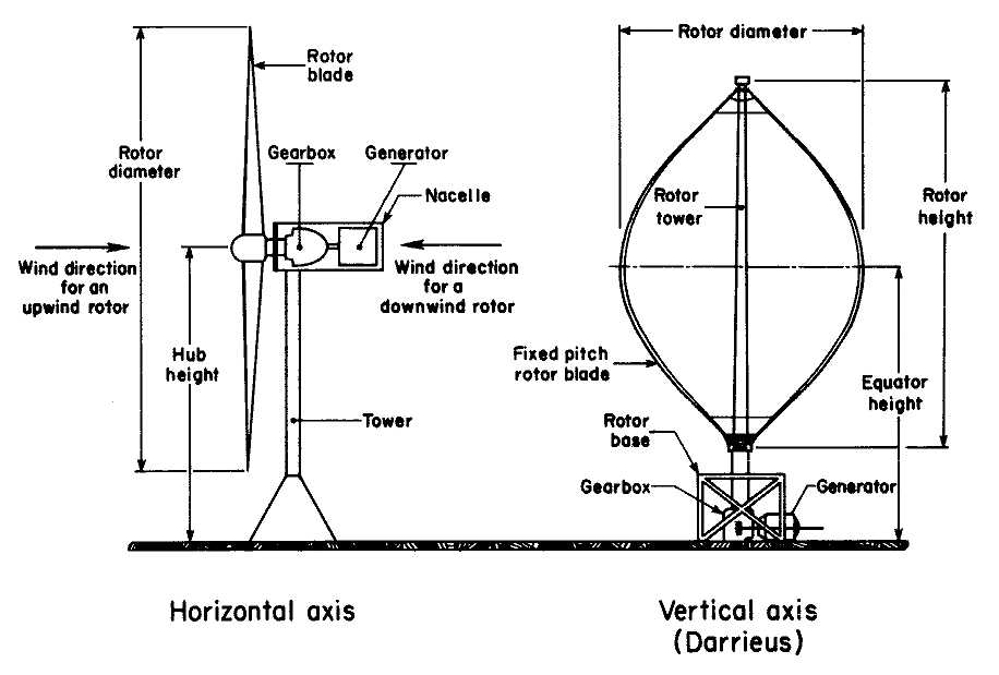
9.1. Vertical axis and horizontal axis wind turbines.
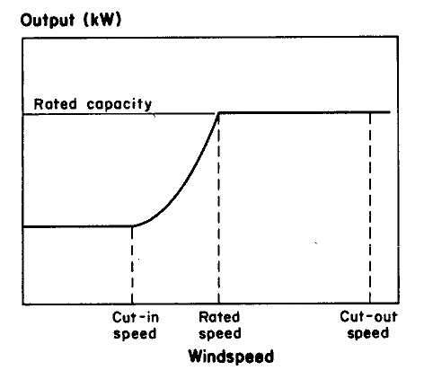
9.2. Windspeed vs. output.
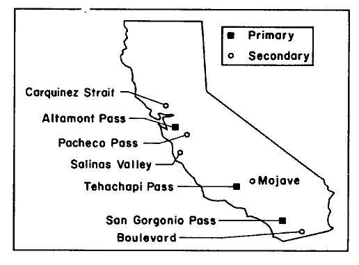
9.3. Major wind farm sites in California.
TEN
Concluding Remarks on the Making of Public Policy
Richard J. Gilbert
The regulation of investor-owned energy utilities was once a matter of applying standardized rules of rate base accounting, with utility management having near total responsibility for system planning and construction decisions. The utility would decide when and what to build. When the project was completed, the utility would submit the bill to its state regulatory commission and it would get paid, with a little profit thrown in for good measure. Utility shareholders had to front the interest costs of construction, but with short lead times for construction and favorable rates, this was not much of a sacrifice. The operation of public utility regulation was not very different from an expense account. Risk exposure to utility shareholders was minimal because expenses were reimbursed according to a cost-plus accounting convention. As long as the utility management remembered to submit the bill for its investments, it would get paid.
This orderly procedure of public utility regulation was shaken by the inflation, environmental constraints, and construction planning errors that characterized the decade of the 1970s. In recent years, regulatory commissions have taken a more active role in the governance of public utility investment behavior. The utility investment programs of the 1970s left a legacy of excess capacity and cost overruns that were unprecedented in the history of the electric power industry. Regulators reacted to the costs of these investments by carefully scrutinizing construction programs and disallowing expenditures that were considered to be "imprudent" or that could not be justified because utility reserve margins were more than sufficient to meet the needs of its service area. Nationwide, regulatory commissions disallowed 9.6% of the expenditures on nuclear plants that were entered into the rate base in the period
1980-86 for a total of $6.6 billion. Of the $6.6 billion, more than half was a penalty for imprudent utility management, and about 33% was based on insufficient need.1 More recent data show an increase in disallowances for nuclear plant construction as a percentage of total investment, with imprudent management as the main cause.2
The experience with the Pacific Gas and Electric Company's (PG&E) Diablo Canyon nuclear power plant summarized by Cox and Gilbert in chapter 7 provides a vivid example of the prudence requirements that a utility must bear in this new age of rate regulation. At the same time, the Diablo Canyon experience provides a faint glimmer of hope by introducing into an actual rate case new principles of utility regulation that determine compensation by the performance of the plant and not by its cost. The Diablo Canyon plant had a book cost of $5.7 billion, but this understates its real cost because shareholders were credited with a low rate for interest on construction expenditures. Following a settlement over the amount of expenditures that would be disallowed for imprudent management of the Diablo Canyon project, the California Public Utilities Commission (CPUC) broke with traditional rate base regulation and endorsed a performance pricing plan for the nuclear plant. Rather than paying for the plant with a formula based on its book cost and the cost of capital (the rate base method), the plant is credited with a payment for each kilowatthour it produces. PG&E's shareholders are required to pay the plant's operating, overhead and capital costs.3 The principle is similar to avoided cost pricing for qualifying facilities under Public Utilities Regulatory Policies Act of 1978 (PURPA). But whereas PURPA limits avoided cost (performance) pricing to small power plants and particular technologies with preferred status, the Diablo Canyon nuclear power plant is the largest single utility project that is compensated with a performance pricing scheme.4
The agreement worked out between PG&E, the CPUC, and the California Attorney General in the Diablo Canyon settlement is a significant step forward in the evolution of utility regulation, but there is no doubt that the settlement has exacted a heavy toll on stockholders for alleged imprudent behavior by PG&E management. Assuming that the Diablo Canyon plant achieves a capacity utilization rate equal to the national average for nuclear power plants of 58%, the expected present value of payments under the Diablo Canyon compensation scheme is less than the book cost of the plant by about $2 billion.5 Payments would increase if the plant performs better than the national average, but PG&E shareholders bear the risk of still lower payments if the plant's performance is worse than average.
Under traditional rate base regulation, utility customers pay the costs of a utility project and bear all of the risk. The shifting of risk from rate-payers to the shareholders is an essential component of incentive regulation. This shifting of risk also has extremely important consequences for the amount and type of investments that utilities will be inclined to undertake in the future. Properly designed, incentive regulations encourage investment in projects that minimize cost, including the cost of risk. However, unless properly designed, incentive regulations may encourage utilities to choose investment projects that minimize the risk to shareholders while ignoring unnecessary costs that may be imposed on ratepayers.
Utility managers protest that incentive mechanisms such as prudence reviews and the performance contract established for the Diablo Canyon plant are nothing more than penalties assessed for cost overruns, with no corresponding reward for investments that have unexpected positive results. According to this view, traditional rate-base regulation provided an implicit contract that permitted utilities to invest with assurance of an adequate rate of return in exchange for an obligation to serve the customers in their franchise area under all conditions (see, e.g., the remarks of the CEO of the Southern California Edison Company, Allen, 1986).6 Regulators have responded to this view by pointing to the excessive investment that can be induced when utilities believe that they are protected from risk (see, e.g., National Association of Regulatory Utility Commissioners, 1983). Both sides have valid complaints. If regulation guarantees a fair rate of return for any capital investment, customers have to bear the risks of excess capacity or construction errors. There is
no incentive for utilities to choose their projects carefully and to balance the risk of excess capacity or an inappropriate capacity mix against the costs of underinvestment. However, if utilities are not rewarded for making the right decisions, yet they are punished for their mistakes, they have no incentive to undertake projects that entail some risk, yet have positive expected benefits for ratepayers.
This concern is evident in many of the chapters in this volume. In chapter 6, Mead and Denning review estimates of the costs of alternative electric power sources in California and the western U.S. They conclude that in the near term, imports of surplus energy from the Southwest and the Northwest are economical sources of supply, but for the longer term, baseload fossil-fuel and nuclear plants appear to be cheaper than renewable sources such as wind, solar and biomass.7 Unfortunately, regulators have not dealt adequately with the challenge to establish a system of incentives that will encourage utilities to invest in projects that promise the greatest expected reward for ratepayers. Nationwide, annual expenditures by investor-owned utilities on generating plants have declined from $27 billion in 1982 to less than $12 billion in 1989, and most of that is on plants that were started a long time ago.8 California utilities are committed to adding only 384 MW of new capacity over the period 1988-93 (California Energy Commission, 1989). The reduction in utility construction expenditures is consonant with the adequate reserve margins in most regions of the nation and, in particular, the large reserve margins in the West. However, this reduction in expenditures is also a reflection of the changing patterns of incentives for new capacity investment in the electric power industry. The California Energy Commission (CEC) expects that more than 2,750 MW of electric power production capacity owned by non-utility generators will become operational in California between 1989 and 1992. Factors have operated on the utility industry to shift the incentives for investment in new generating capacity from traditional utility suppliers to non-utility sources of power. PURPA encourages non-utility investment, while active implementation of the prudence doctrine has discouraged utilities from undertaking the financial risks of large construction programs. This has led to greater diversity in the institutional structure of the electric power industry and in the size mix of new power investments. Power plants that are qualified facilities (QFs) under PURPA range from a few kilowatts to hundreds of
megawatts in size. The roster of new power plant additions in California now includes names such as the Teddy Bear Wash and Dry of Capitola and the Oroville Taco Bell (each 10 kW of cogeneration), Shell (48 mW of natural gas for enhanced oil recovery), and Signal Energy Systems (55 mW of biomass), alongside of the long-delayed Diablo Canyon and San Onofre nuclear power units.9
The dramatic consequences of PURPA and related regulatory incentives for the diversity in plant size and ownership in California have not been matched by an increase in the diversity of fuel supply. Most of the power plant investment that has been stimulated by PURPA is gas-fired cogeneration. Wind power enjoyed a period of rapid expansion, but this came to almost a complete halt after the expiration of state and federal tax subsidies. PURPA has succeeded in encouraging some investments in biomass and solar power, but this has been a small fraction of total supply. As of 1980, about 60 percent of qualifying investment in the combined PG&E, Southern California Edison (SCE) and San Diego Gas & Electric California (SDG&E) service areas has been cogeneration, most of which is gas-fired. Excluding wind power, the fraction of QF power that is cogeneration is 72 percent. (Source: PG&E, 1989; SCE, 1989; SDG&E, 1989.)
Most utilities have been content to rest on their comfortable reserve margins, or to enlist with the army of independent power producers. The margin of excess production capacity in the West is sufficient to put off the initiation of major construction programs until the middle of the 1990s. Demand management programs can extend the day of reckoning, but unanticipated increases in the rate of demand growth would have the opposite effect. In California, non-utility QF generators have been the electric power supply source of the 1980s. In 1988, QFs and self-generators accounted for about 8% of total generation in California. The CEC predicts that by the year 2000 this number will increase to 15% (CEC, 1989).
Utility commissions have made only a partial response to the challenge to eliminate the distortions caused by traditional rate regulation while rebuilding incentives for baseload utility investments. One of the problems of conventional rate regulation is that regulators, by setting rates to recover the average cost of supply, are likely to drive a wedge between the rates that customers pay and the economic (marginal) cost of supply. The chapters by Friedman (chapter 2) and by Gilbert and Henly (chapter 4) emphasize the desirability of using nonlinear prices to improve on the efficiency of rate regulation. Regulated prices compensate utilities for the cost of production and guide consumers in their energy purchase decisions. Compensatory prices need not provide consumers
with the correct information about the real cost of energy. Utilities (both electric and gas) in the Western United States invested in the 1970s in anticipation of a high rate of growth in demand that was not realized. The consequence was a large amount of capacity above normal reserve requirements. This excess capacity, coupled with cost overruns and declining fuel prices, resulted in a situation where the average cost of generation in the West in 1989 is far above the marginal cost of that power, and this relationship is expected to continue for several years. Economic theory dictates that efficient prices should be as close as possible to the marginal cost of production. Under California rate-making procedures, regulators set compensatory prices that increase with the amount that is consumed, with the result that retail energy prices in 1989 are far in excess of marginal production costs. Gilbert and Henly estimate that the excess of the price of electricity over its marginal cost will result in a loss of economic value to Californians of about $1 billion per year over the period 1987-2003.
Friedman, Gilbert and Henly suggest that these distortions can be eliminated with use of a two-part pricing scheme. If marginal cost is below the average cost of production, the retail price can be held close to marginal cost and customers can be assessed an access fee to make up the difference between total cost and revenue receipts. If marginal cost is more than average cost, customers can receive an access credit which would appear as a deduction from their monthly bills. Friedman points to the potential that marginal-cost based rates may give the wrong signal to electricity consumers. If higher marginal electricity costs are likely in the near future because reserve margins will shrink and fuel prices increase, then low prices today could deter consumers from making demand-conserving investments that would be profitable at expected prices. The counter to this argument is that prices today which greatly exceed marginal cost are a certain compromise of economic efficiency. If marginal costs are expected to rise, this information can be communicated to consumers, who should plan accordingly.
In chapter 3 Gilbert describes some of the changes in utility regulation that have followed from the Public Utility Regulatory Policies Act of 1978 and suggests a way to usher the industry into a more competitive era. An essential component of greater competition in electric power is a move toward competitive procurement of new supply. Competitive procurement can take many forms, ranging from increased reliance on power pooling agreements among utilities to mandatory auctions for new sources of supply. These auctions may be conducted by regulatory commissions and may. include bids for demand-side management as well as new generation sources.
The greatest departure from traditional ratemaking would allow retail consumers to conduct bids for supply sources. Recent changes in the
regulation of natural gas provides one model for a more competitive electric power sector. In chapter 5 Russo and Teece describe the changes that have occurred in natural gas regulation in California. Natural gas supply has been "de-bundled," allowing industrial customers to contract separately for natural gas supply and for the transportation of gas from its source to the customer. Utilities are required to provide transportation services. A customers may choose to stay in a "core" market, where he has a guaranteed supply and pays a "bundled" rate for natural gas and transportation. Those who elect to participate in the "non-core" market have the flexibility to contract for cheaper sources of supply, but cannot rely on the local gas distribution company for guaranteed service.
The experience with natural gas deregulation provides a stimulating, but imprecise model for deregulation of the electric power industry.10 It is imprecise because the technology of natural gas distribution differs substantially from the technology of electric power, where network interactions are more complex and there is more reliance on the coordination of transactions. Electric power must be supplied on demand, and this requirement makes instantaneous coordination of supply and distribution a necessity.
Despite these crucial differences, present developments in electric power regulation suggest an increasing emphasis on competitive procurement and contractual relations, as has occurred in the natural gas industry. Competitive procurement of power sources inevitably implies a movement from regulation as an administration process to regulation through formal contractual obligations. Contracting is not a panacea. There are enormous problems associated with contracting, including defining the conditions of the contract, the obligations of the parties, negotiation of changes to the contract, unforeseen events, administering and monitoring contract performance, and the method of payment. The difficulties are so severe that is it highly likely that competitive procurement will evolve into a system of quasi-regulation, where a small number of qualified suppliers engage in periodic negotiations with the public utility commission (similar to rate hearings) to determine the obligations of supply and the amount of payment.
One particularly interesting regulatory experiment that involved both competitive procurement and the development of new sources of supply was the California and federal tax subsidies for renewable sources of energy. PURPA introduced competition in electric power supply by requiring utilities to purchase wholesale power from certain qualified facilities at rates determined by regulatory review and based on the value of power that is "avoided" as a result of the purchase. The
combination of guaranteed access under PURPA, federal and state tax subsidies, and generous long-term contracts for the procurement of power established by the CPUC (the Standard Offer 4 contract) provided powerful incentives for the development of alternative energy sources in the state. A good example of the response to these incentives is the development of wind power in California. The installed capacity of wind power in the state grew from about 7 MW in 1981 to 1,141 MW by the end of 1985. This exceeded even the goal of the California Energy Commission and established the largest wind power program in the world.
In chapter 9 Blumstein, Cox, and Gilbert argue that targeted tax subsidies accomplished the objective of spawning a wind industry, but at too great a cost. By the end of 1987, cumulative investment in wind power in the state was in excess of $2 billion. Substantial progress was made in reducing the cost of wind power from about $4,000 per kilowatt to an estimated $1,100 per kilowatt for the newest machines. However, despite substantial technical progress, wind power is still not expected to be a competitive alternative to fossil fuels over the near term without subsidies. Equipment reliability and erratic wind patterns contribute to a low rate of capacity utilization for wind power, rarely in excess of 18 percent. If wind power is compared to a conventional base load power plant with a capacity factor of 60%, the effective cost per kilowatt is in excess of $3,600 per kilowatt for the newest vintage of machines. This compares to about $2,600 per kilowatt for the Diablo Canyon nuclear plant and $1,000-$1,500 per kilowatt for modern baseload fossil units. Wind power has the advantage of lower operating costs, but this is not sufficient to compensate for the higher capital costs at anticipated fossil-fuel prices. In addition, Mead and Denning argue that the value of the electricity that has been produced by wind in California is less than the average value of power from baseload plants because strong winds do not coincide with the time of peak electricity demand (at least at Altamont Pass, the wind farm region with largest installed capacity).
California wind energy provided valuable information about the potential for wind as an energy source and succeeded in exploiting economies of scale and experience. However, the end result of the program was an industry that was still too costly to compete with other sources of supply in the absence of targeted subsidies. The information that was produced is useful, but a program of much smaller scale could have provided similar information at much less cost. This conclusion contrasts with the findings of Cox and Gilbert that it was economic to complete the Diablo Canyon nuclear power plant given the information that was available in 1981 or later. The important difference is that the Diablo Canyon project is indivisible—it is either completed or canceled. With the large amount of capital costs that were already sunk by 1981, it was
prudent to carry the plant to completion. Wind power is not an indivisible investment. When sufficient information was available to predict that wind power would not be an economic alternative without subsidies, the subsidies should have been terminated. This did happen, but a more sensible approach would have been to move more slowly in the development of wind power and to cancel the subsidies by 1984, when it was apparent that wind power would not be an economic alternative source of supply at existing fuel prices. A main objective of California regulators is the encouragement of a diverse electric power supply system, in which wind power was expected to play a significant role. Mead and Denning argue that unconventional sources of supply including solar, wind, and biomass are unlikely to be attractive alternatives to conventional fossil fuels over the next decade, and new hydropower sites within the state are limited. Mead and Denning claim that even allowing for environmental impacts, nuclear power and coal are more economic sources of supply for California than the renewable alternatives. Yet no new investment in nuclear power can be expected given social opposition and the financial risk to regulated, investor-owned utility companies and coal-fired power has to be imported into California from distant regions where the environmental impacts and economic costs of further development are likely to result in opposition to new power plant siting. PURPA has stimulated new sources of supply in California, but most of these sources are powered by conventional fossil fuels, with gas-fired co-generation being the largest contributor. With the exception of the promise of advanced-cycle gas-fired turbines, which may offer a source of supply with acceptable cost, low emissions, and relatively easy siting (see Williams and Larson, 1989), the prospects for new, diversified sources of energy for California and the West are not encouraging.
Against this rather grim prospect, it is not surprising that there has been a renewed emphasis on the value of demand management as a "supply" source for the 1990s. Proponents of increased efforts to exploit the benefits of energy conservation point to the potential to generate energy savings through end-use investments at a price per kilowatt-hour (or per barrel of oil equivalent) that is less than the cost of producing energy to meet projected demands. A question facing policymakers for the 1990s is why these cost-effective programs are not undertaken by consumers, or why private firms have not succeeded in exploiting the benefits of energy conservation by entering into arrangements with consumers to lower their energy bills. An argument in favor of an aggressive program to support energy conservation is that demand management eliminates many of the harmful environmental impacts of new sources of supply. Mead and Denning find that the environmental impacts of coal and nuclear power add only a relatively small amount to their private
costs; however, this analysis implicitly assigns a zero price to impacts that are not included and therefore is likely to underestimate true social costs. Nonetheless, one should also note that, in California, most customers already pay a price for electricity that far exceeds its (private) cost of generation. (Gilbert and Henly find that consumers pay an average of about 9 cents per kilowatt-hour for electricity that costs about 2.5 cents on the margin to produce). This means that most customers already face an incentive to conserve electricity that is substantially greater than the private marginal cost of power and may even exceed its social cost including environmental impacts.
Notwithstanding the large gap between price and marginal cost, John Quigley finds examples where clearly attractive opportunities for energy conservation are not exploited (chapter 8). Expressed in dollars per barrel of oil-equivalent savings, Quigley finds several programs with estimated present value costs of energy saved that are less than $20 per barrel. In one case, a seasonal pilot light program, the energy saved was estimated to cost less than $1 per barrel of oil-equivalent! No doubt the potential for these programs to contribute to our energy future has not been fully exploited. Furthermore, the erosion of reserve margins and higher fuel prices that can be expected in the future will close the gap between the average and marginal costs of electric Power. It will not be long before utilities will be forced either to subsidize demand management programs or to invest in new baseload plants. For many utilities, subsidizing demand management programs will be less onerous than convincing regulators of the need to site new generation facilities.
However, attaining the goal of efficient utilization of energy will not be an easy task. There are many reasons why consumers fail to minimize the cost of energy consumption. One reason is imperfect information. Another is that in many circumstances, the person who decides the amount of energy that will be consumed (or the type of energy-using equipment that is installed) is not the same as the person who pays the bill. Yet another reason is that for many consumers, energy is still not a large enough component of their total expenditures to justify extraordinary diligence in its use.
Some, but not all, of these reasons why consumers are not efficient energy consumers are reasons why regulators may wish to pursue programs to subsidize demand management. The difficulty with this approach is that subsidies will encounter many of the problems that keep consumers from exploiting end-use efficiency. Quigley found that many of the demand management programs that have been promoted in California are unlikely to be winners by anyone's calculus. Some of these programs had present value costs of energy saved in excess of $50 per barrel
of oil equivalent. If regulators are going to implement demand management programs that promote efficient use of all of society's resources, it will be necessary to take extreme care to separate the programs that provide real savings from those that may save energy, but at an unacceptable price.
The chapters in this book provide a record of the consequences of regulatory innovation and suggest what may lie ahead in the regulatory energy supply sector of our economy. The record is mixed. Some of the innovations, such as targeted tax subsidies for demand conservation and for renewable energy supply, accomplished their objectives but at a cost that could not and should not be sustained. Energy credits created tax-sheltered investment programs that established a costly wind program that did not succeed in attracting capital for new investment after the credits were discontinued. John Quigley found that a disproportionate share of residential conservation credits were used by wealthy taxpayers, and much of that for investments in pools and spas. The introduction of new competition into regulated energy markets has also enjoyed only mixed success. Non-utility generators are the dominant source of new supply for California in the 1990s, yet most of this supply has a price that moves with the cost of fossil fuels and therefore provides inadequate insurance to California ratepayers against petroleum and natural gas price increases. Yet there is also hope that by encouraging new sources of supply and new types of suppliers, energy markets will become more resilient, because the market will integrate diverse judgements. The experience with nuclear power in the U.S. is an example of the risk of too much reliance on a course of action that is derived from a consensus view of traditional utility investment behavior.
The path to successful coordination of the different actors that have entered the regulated energy markets will not be easy. There will be problems in achieving access to markets, in coordinating supply decisions, and in balancing private gains against social costs. Although there are as many futures for the regulated energy markets as there are people to make forecasts, it seems certain that the industry will continue to move away from its historical emphasis on cost-plus contracting, that there will be an increased reliance on incentive contracts and competition in the procurement of new supply, and that utilities and regulators will look toward demand management as a way to postpone the inevitable task of siting new baseload generation facilities. As the utility industry adapts to the newly competitive nature of these markets, it will be possible to repair the existing regulatory structure with its disincentives for new investment, and the industry can confront the challenges that lie ahead.
REFERENCES
Allen, Howard P. (1986). "The Changing Electric Utility Industry: The Customer Comes First," Executive Conference, Cambridge Research Associates, Houston, Texas, January 28.
California Energy Commission (1989). "Electricity, 1988 Report," P106-88-001, June.
California Public Utilities Commission (1988). "PUC Approves Settlement of the Diablo Canyon Case," PUC News , December 19.
Joskow, E, and R. Schmalensee (1986). "Incentive Regulation for Electric Utilities," Yale Journal on Regulation , 4:1-49.
National Association of Regulatory Utility Commissioners (1983). "Incentive Regulation in the Electric Utility Industry," Washington, D.C.
Oak Ridge National Laboratory (1987). "Prudence Issues Affecting the U.S. Electric Utility Industry," ORNL/Sub/86-56559/1, December.
Oak Ridge National Laboratory (1989). "Prudence Issues Affecting the U.S. Electric Utility Industry, Update: 1987 and 1988 Activities," ORNL/Sub/86-56559/1, February.
Pacific Gas and Electric Company (1989). "Cogeneration and Small Power Production Quarterly Report to the California Public Utilities Commission," Third quarter.
Pierce, R. (1989). "Using the Gas Industry as a Guide to Reconstituting the Electricity Industry," Columbia University School of Law, working paper No. 35.
Southern California Edison (1989). "Cogeneration and Small Power Projects, Quarterly Report," Third Quarter.
Standard and Poor's (1990). Industry Surveys , January.
Williams, R., and E. Larson (1989). "Expanding Roles for Gas Turbines in Power Generation," in T. Johnson, B. Bodlund, and R. Williams (eds.), Electricity: Efficient End-Use and New Generation Technologies and Their Planning Implications . Lund, Sweden: Lund University Press.
INDEX
A
Abandonment payments, 376 n.3
Accelerated cost recovery system (ACRS), 354 -55, 361
Access fees, 380
ACRS (accelerated cost recovery system), 354 -55, 361
Aeroderivative turbines, 378 n.7
AFBC (atmospheric fluidized-bed combustion), 206 , 207
AFUDC (allowance for funds used during construction), 64 -65, 96 n, 264 ;
at Diablo Canyon, 260 , 263 -67, 269 , 270 -71, 273 , 276 , 277 , 277 n. 19, 278 -79;
"replacement," 264
AGA (American Gas Association), 120 n, 128
AIA (American Institute of Architects), 308
AIF (Atomic Industrial Forum), 229
Air conditioners, 95 n. 16;
alternatives to, 18 -19;
direct load management and, 49 -50, 53 ;
NBS criteria for home, 308 ;
solar-powered, 298 ;
wind-powered, 298 . See also Space conditioning
Air pollution, 9 , 43 , 203 -4;
fuel oil and, 155 ;
nuclear power and, 226 . See also Acid rain;
Greenhouse effect;
Particulates
Alaska: gas production of, 126 -27;
oil of, 190
Alaska pipeline, 68 n
Alberta: tar sands of, 211
Alcoa, 69
Alcohol: as gasoline substitute, 212
Alquist Bill, 294
Altamont Pass wind farms, 219 , 221 -22, 353 , 382 ;
energy storage at, 223 ;
windmills of, 356
Aluminum industry: growth of, 69 ;
and power demands of Pacific Northwest, 194
American Electric Power Company, Tidd plant of, 207
American Gas Association (AGA), 120 n, 128
American Institute of Architects (AIA), 308
American Insurance Association, 309
American Society of Heating, Refrigeration, and Air Conditioning Engineers. See ASHRAE
Appalachian-Illinois gas-producing area, 127 n. 15
Appliances, household, 34 ;
efficiency standards for, 2 , 291 n. See also Air conditioners;
Freezers, electric;
Water heaters
Aquifers, energy stored in, 224
Arizona: electric power in, 199 ;
electric power between California and, 200 ;
electric power from Oregon to, 197 ;
nuclear power plants of, 199
Arrays, wind-power, 221
ASHRAE (American Society of Heating, Refrigeration, and Air Conditioning Engineers), 90 -75, 308 -9
Athabasca Tar Sands, 211
Atmospheric fluidized-bed combustion (AFBC), 206 , 207
Atomic Industrial Forum (AIF), 229
Auctions, power-source, 380
Audits, energy conservation-related home, 305 , 306
Automobile industry, 67 ;
fuel-economy standards mandated for, 291 n, 292 ;
new-model costs in, 69
Avoided costs, 77 , 77 n, 213 , 215 , 217 , 222 , 376 ;
and Diablo Canyon, 271 -72;
negative, 216 ;
at PG&E, 222 ;
B
Barkovich, Barbara, 10 n
Baseline, 162 n.57
Baseline allowances, 135 n.30, 162
Baseline rates, 30 -31, 35 -36, 95 , 95 n. 16, 105 , 108 , 138 , 139 , 162 . See also Increasing block rates;
Lifeline rates
Baseline tier quantities, 14
Baseload plants, 65 , 69 , 70 ;
fuels for,191
Battery energy storage, 223
B.C. Hydro (British Columbia Hydro and Power Authority), 195 -96, 197 , 201 -2, 234
Bechtel Corporation, 210
BEPS (building energy performance standards), 309
Biomass, combustion of, 5 , 73 n.6, 203 , 214 , 224 , 232 , 236 , 378 , 379 , 383 ;
synthetic gas from, 378 n.7
Block rates, 31 , 52 , 88 n.6, 107 , 125 -26. See also Declining block rates;
Increasing block rates
Block tariffs, 84
Blowouts, natural gas well, 130
BOCA (Building Officials and Code Administrators International), 309
Bonneville Power Administration. See BPA
BPA (Bonneville Power Administration), 192 , 197 , 233 -34, 237 ;
intertie access policy of, 192 , 195 -96, 198 , 201 , 202 , 234 ;
obligations of, 198
Brazil: ethanol as motor fuel in, 212
Breckenridge coal liquefaction plant, 208
British Columbia: power to California from, 187 , 234 . See also B.C. Hydro
British Columbia Hydro and Power Authority. See B.C. Hydro
Brownouts, 86
Building codes, energy conservation-compatible, 308
Building energy performance standards (BEPS), 309
Building Officials and Code Administrators International (BOCA), 309
Buildings. See Construction;
Homes
Burlington Northern, Inc., 133
Burner-tip rates, 121 , 121 n;
for noncore sector, 145
Butane, 304
Bypass, 3 , 4 , 8 , 79 , 89 , 91 , 99 , 103 . See also Cogeneration;
Self-generation
C
CAES (compressed-air energy storage), 223 , 224 , 236
California: electric power sources in, 5 , 187 -259 passim;
energy-conserving building standards of, 310 -16;
energy policy in, 14 -18 (see also CEC; CPUC);
energy utilities of, 10 -62 passim (see also PG&E; SCE; SCG; SDG&E);
in-state alternative power sources of, 202 -31 passim;
natural gas industry of, 120 -86 passim;
power imported by, 192 -202;
tar sands of, 211 ;
utility prices in, 10 -62 passim
California Commission on Housing and Community Development (HCD), 310
California Energy Commission. See CEC
California gas-producing area, 127 n. 15
California Public Utilities Commission. See CPUC
Cambridge Energy Research, Ltd., 227
Canada: natural gas exported from, 131 -32, 133 , 134 , 135 . See also Alberta;
British Columbia;
Ontario
Capacity payments, 222
Carbon dioxide, 226
Carbon monoxide, 226
Carter, Jimmy, 353
Caulking, energy-conserving, 292 , 293 , 305 , 306 . See also Insulation;
Weatherization
Caverns, energy stored in, 224
CEC (California Energy Commission), 14 , 20 -21, 74 , 88 ;
and AB 163 provisions, 313 -14;
and demand charges, 41 ;
energy forecasts of, 187 -92;
and qualifying facilities, 216 -17;
and tax credits, 366 ;
Title 24 standards of, 311 -13;
and wind energy, 347
Cement industry, 67
Cereals: ethyl alcohol from, 212
CG prices. See City-gate (CG) prices
Charles Rivers Associates (CRA), 302
Chernobyl nuclear power plant, 235
Chrysler, 69
Circulating bed PFBC, 206
City-gate, 121
City-gate (CG) prices, 122 , 140 n.36, 148 -49, 162
Clarke, Richard A., 217
Class allocation, 14 , 17 , 54 , 92 . See also EPMC (equal-percentage of marginal cost) pricing
Coal, 5 , 201 , 206 -10, 232 , 235 , 236 ;
electricity generated by, 188 , 193 , 203 , 376 n. 1, 383 ;
environmental aspects of, 8 , 43 , 204 , 383 ;
as fuel oil substitute, 206 , 226 -27, 228 , 229 -30;
gasification of, 206 , 208 , 209 , 237 (see also GCC);
liquefaction of, 208 -9, 237 ;
as natural gas substitute, 206 ;
as nuclear power alternative, 268 ;
PIFUA and, 137 ;
price of, 188 ;
social costs of combustion of, 229 , 235 ;
Southwest dependence on, 199 , 200 , 202 ;
synthetic gas from, 378 n.7;
versatility of, 206 ;
world reserves of, 206
Coal gas, 122
Coase, R.H., 33
Cogeneration, 73 -75, 76 , 89 -90, 91 , 140 , 160 -61, 269 n.11, 277 , 379 , 383 ;
in Kern County, Calif., 156 . See also Self-generation
Cogeneration plants: as qualifying facilities, 193
Colorado: electric power in, 199 ;
natural gas to California from, 153
Colorado River, 199
Combined-cycle generating plants, 269 n.11
Commercial class, 101 -2
Commercial impracticability, 130
Common carriers, natural-gas pipelines as, 131
Commuter railroads: and CPUC, 135
Competition: rate regulation and, 8
Compressed-air energy storage (CAES), 223 , 224 , 236
Connection accounts, 34 -36, 52
Connection charges, 14 , 34 , 35 n.38, 36
Connection credits, nonrefundable, 34 , 34 n, 35 , 36
Consolidated Edison, 21
Construction: energy-conserving standards for, 20 , 20 n, 291 n, 294 , 307 , 308 -16
Consumerism, 147
Consumers. See Energy consumers
Contract carriage, 4 , 8 , 125 , 131 , 132 , 133 , 145 , 153 -56, 162
Cooling fans, energy-conserving, 296
California natural gas, 145 -46
Cost-of-service estimates, 143
Cost recovery, utility, 96 -99, 103 -8
CPUC (California Public Utilities Commission), 10 , 12 -18, 24 , 25 , 32 , 92 , 120 -21, 134 , 135 -47, 152 , 161 -63;
authority of, 135 ;
and baseline pricing, 35 -36, 36 n.39;
and block rates, 36 ;
and cogeneration, 160 -61;
and contract carriage, 145 , 155 , 158 ;
and core/non-core customers, 4 ;
and Diablo Canyon nuclear power plant, 271 -72, 376 -77;
and EPMC method, 27 -31, 33 , 106 ;
"gamesmanship" of, 144 , 163 ;
and gas-fired power plants, 137 ;
and Kern County dispute, 156 ;
and limit pricing, 158 ;
members of, 17 , 28 (see also CPUC, staff of);
and prioritization, 158 ;
Public Staff Division (PSD) of, 142 -44;
and qualifying facilities, 156 , 215 , 217 ;
and rate design, 36 -50;
Rate Design Branch of, 15 -16;
and residential TOD pricing, 45 -46;
and revenue allocation, 24 -36;
social goals of, 135 , 138 , 140 , 148 , 161 ;
solar en-
ergy encouraged by, 304 -5;
standard offers of, 74 , 79 , 215 , 216 , 355 , 382 ;
and subsidization, 88 n.8;
and telecommunications pricing, 162 ;
and two-part tariffs, 34 ;
and value-of-service structure, 138 , 139 -45;
CRA (Charles Rivers Associates), 302
"Cream skimming," 139
Cross-subsidization, 80 , 135 , 136 , 138 -39, 141 , 143 , 144 , 152 , 158 , 162
Crude oil. See Petroleum
Crude Oil Windfall Profits Act, 292
Cut-outs, high-wind, 221
D
Darrieus windmills, 350 , 351 , 354
Declining block rates, 3 , 32 , 36
Decommission costs, 226
Delivered prices, natural gas, 121 n
Demand, consumer, 48
Demand charges, 14 , 37 -42, 52 , 53 -54
Demand elasticities, 26 , 27 n, 31 , 91 , 93 , 98 -99
Demand management programs, 379 , 384 -85
Demand Subscription Service, 49 n.62
Department of Energy. See Energy, U.S. Department of
Depletion allowance, fuel, 220 n.18
Depreciation, 96 ;
SCG and, 142 ;
wind power and, 354 -55
Derived demands, 18 -19
Deukmejian, George, 295
Diablo Canyon nuclear power plant, 5 -6, 189 , 260 -89 passim, 379 ;
capacity of, 74 , 192 , 192 n, 269 , 269 n.12;
construction of, 189 , 227 -28, 233 , 260 , 275 , 278 , 279 , 382 -83;
cost of, 65 , 228 , 260 -67, 269 -80, 376 -77;
and earthquake hazard, 260 , 278 ;
errors in construction of, 278
Direct-flash dry steam, 225
Direct load management, 14 , 49 -50, 53
Disaster insurance, 21
Dispatchability, 216
Distribution costs, 41 , 41 n.49
Distribution margins. See Gross margins
Dividends, for electric consumers, 95
Dixie Valley geothermal plant, 225
DOE. See Energy, U.S. Department of
E
Earthquake, as Diablo Canyon hazard, 260 , 278
ECABF (energy cost adjustment), 30 n.28
ECAC (energy cost adjustment clause), 17
Economic Opportunity, California Department of, 292
Economic Recovery Act, 354
Efficient price, 86 , 86 nn.3,4
EIA (Energy Information Administration), 318
Elasticities, demand, 26 , 27 n, 31 , 91 , 93 , 98 -99
Electricity: air conditioners and, 22 ;
NBS criteria for residential, 308 ;
pricing of, 8 ;
residential, 33 -34;
TOU pricing for, 42 . See also Electric power
Electric power: California sources of, 187 -259 passim;
consumption of, 188 , 189 , 231 ;
market structure for, 66 -70;
rate reform and, 84 -119;
storage of, 203 ;
variation of marginal source, 140 n.37. See also Electricity;
Hydroelectric power
Electric Power Research Institute (EPRI), 207
Energy: cost of, 14 , 316 -19;
efficiency standards for, 20 ;
storage of, 223 -24, 236 . See also Electric power;
Energy conservation;
Environmentalism;
Fuels;
Geothermal energy;
Hydroelectric power;
Nuclear power;
Solar power;
Wind power
Energy, U.S. Department of (DOE), 41 ;
and BEPS, 309 ;
and residential energy conservation, 292 -93
Energy conservation, 6 -7, 8 , 188 , 202 , 204 -6, 261 n, 383 -85;
California utilities and residential, 304 -8;
CPUC-mandated, 149 ;
encouragement of in California, 292 , 293 , 294 -96, 297 -300, 303 -8, 310 -16, 319 ;
federal impetus to, 291 -94, 296 -97, 300 -303, 308 -10, 319 ;
natural gas industry and, 124 ;
and new construction, 20 , 20 n, 291 n, 294 , 307 , 308 -16;
and nuclear
power, 268 ;
and petroleum prices, 204 -5;
residential, 290 -346 passim
Energy Conservation and Production Act, 291 n, 309
Energy Conservation in Existing Buildings Act, 292
Energy consumers, 18 -24;
and block rates, 32 n.34
Energy cost adjustment (ECABF), 30 n.28
Energy cost adjustment clause (ECAC), 17
Energy Information Administration (EIA), 318
Energy Policy and Conservation Act (EPCA), 291 n, 309
Energy rate adjustment mechanism (ERAM), 17
Energy Reorganization Act, 291 n
Energy Resources Conservation and Development Commission (ERCDC), 310
Energy Security Act, 293
Energy Tax Act, 354
Energy Tax Credit (ETC), 6 -7, 213 , 218 , 219 -20, 222 , 292 -300, 319 , 347 -49, 354 -63, 363 n.16, 366 , 368 , 382
Enhanced oil recovery (EOR) market, 156 , 157 n, 158 -61
Entry fees, 33 -34
Environmentalism, 8 -9, 11 , 43 , 375 , 383
vs. utility expansion, 64
EOR (enhanced oil recovery) market, 156 , 157 n, 158 -61
EPCA (Energy Policy and Conservation Act), 291 n, 309
Episode days, 141
EPMC (equal-percentage of marginal cost) pricing, 13 , 34 , 46 , 98 -106, 108 ;
and optimal uniform pricing, 27 -31
EPRI (Electric Power Research Institute), 207
Equal-percentage of marginal cost pricing. See EPMC pricing
ERAM (energy rate adjustment mechanism), 17
ERCDC (Energy Resources Conservation and Development Commission), 310
ETC (energy tax credits), 6 -7, 213 , 218 , 219 -20, 222 , 292 -300, 319 , 347 -49, 354 -63, 363 n.16, 366 , 368 , 382
Ethyl alcohol, as gasoline substitute, 212
Expected costs, 86
Externalities, positive, 349
Exxon Corporation: PVEA and, 293
F
FBC (fluidized-bed combustion), 206 -8, 229
Federal Communications Commission, 73
Federal Energy Administration, 41 ;
and energy conservation, 291 n
Federal Energy Agency, 317
Federal Energy Regulatory Commission. See FERC
Federal Power Commission (FPC), 122 -23. See also FERC
Federal Trade Commission, 122 , 123
FERC (Federal Energy Regulatory Commission), 73 n.7, 120 , 123 , 125 -26;
and alternative power sources, 214 -15;
and California, 135 , 135 n.29;
and contract carriage, 155 , 158 ;
Order 380 of, 129 n;
Order 436 of, 125 , 125 n.12, 131 ;
and qualifying facilities, 193 n
Firm capacity imports, 193
Firm energy, 193 , 194 , 199 , 233 , 234
Fitchburg Gas & Electric Company, 70
Flat rates, 36
Flat tariffs, 97 n
Floor payments, 376 n.3
FloWind Partners 1984, 360 -62
Fluidized-bed combustion (FBC), 206 -8, 229
Force majeure clauses, 130
Fossil fuels. See Coal;
Fuel Oil;
Natural gas;
Petroleum
Foster Associates, 317
FPC (Federal Power Commission), 122 -23. See also FERC
Freezers, electric, 95 n. 16
Fuel adjustment clauses, 15
Fuel oil, 5 , 11 , 201 , 232 , 234 ;
California conservation of, 307 -8;
coal as substitute for, 206 ;
cost of, 188 , 190 , 262 , 268 , 269 , 271 , 272 -80, 363 , 365 -66, 366 n.21, 367 ;
Diablo Canyon project and, 6 ;
distillate, 124 ;
electricity generated by, 43 , 188 , 191 , 198 , 199 , 203 , 230 -31, 268 , 269 ;
natural gas and, 128 , 133 , 137 , 139 -40;
as PG&E fuel, 39 n.46;
and pollution, 155 ;
regulation of, 122 ;
of San Joaquin Valley, 153 ;
SCE and, 141
Fuels: finite supply of, 54 ;
synthetic, 137 ;
as utility expense, 2 , 3 , 15 , 17 , 25 , 54 ,
64, 87 -90, 92 , 135 -36. See also Bio-mass;
Coal;
Energy;
Fuel oil;
Gasoline;
Natural gas
Furnaces, 21 ;
G
Gamson, David, 10 n
Gas. See Coal gas;
Gasoline;
Natural gas;
Synthetic gas
Gasification combined-cycle (GCC), 206 , 208 , 235
Gasohol, 212
Gasoline: coal converted to, 206 , 209 -10, 237 ;
natural gas converted to, 210 , 237 ;
substitutes for, 212 ;
taxes on, 205
GCC (gasification combined-cycle), 206 , 208 , 235
General rate cases, 15 -18, 24 , 51
Generators, windmill, 351 -52
Geothermal energy, 39 n.46, 203 , 225 , 232 , 236 , 237 , 268 ;
federal encouragement of, 291 n
Germany: gasoline from coal in, 209 -10
Geysers, The, 225
Glass industry, 67
Glazing, 316 . See also Storm windows/doors
GN rates, 142 n.41
Great Plains coal gasification plant, 209
Greenhouse effect, 204 , 226 , 229
Gross margins, 147
H
Hausker, Karl, 10 n
HCD (California Commission on Housing and Community Development), 310
Heating, residential: NBS criteria for, 308 ;
solar, 298 ;
wind-powered, 298 . See also Furnaces;
Space conditioning;
Water heaters
Heat pumps, energy-conserving, 296
Heat rate, 268 , 270 , 270 n. 14, 272 , 364 , 364 n.17;
cogeneration and, 277
Heat transfer: NBS criteria for, 308
Heber, Calif., geothermal plant, 225
Helms pumped-storage facility, 224
Holding companies, electric power industry, 66
Homes: energy-conserving improvements to, 291 n, 292 -96, 298 , 302 -6. See also Weatherization
Hoover Dam area, hydropower system of, 193
Hopkinson tariffs. See Demand charges
Hot tubs, solar-heated, 6
Housing and Community Development, California Commission on (HCD), 310
Housing and Urban Development, U.S. Department of, 309 ;
and energy-conserving construction, 310 ;
responsibilities of, 309 -10
Houston Natural Gas Corporation, 133
HUD. See Housing and Urban Development, U.S. Department of
Hugoton-Anadarko gas-producing area, 127 n.15
HVAC. See Air conditioners;
Heating, residential;
Ventilation
Hydroelectric power, 11 , 135 , 188 , 199 , 203 , 232 , 237 , 268 , 383 ;
of British Columbia, 234 ;
on Colorado River, 199 ;
imported, 5 ;
of Pacific Northwest, 192 -93, 194 -95
Hydro spill, 216
I
ICBO (International Conference of Building Officials), 308 , 309
ICF-Mathematica, 302
IEES (International Energy Evaluation System), 318
IEW (International Energy Workshop), 318
Ignition devices, intermittent, 306
Import tariffs, on petroleum, 205
Incentive regulations, 377
Increasing block rates, 3 , 31 n.32, 87 -88, 95
Indonesia, residual oils of, 139
Infant industries, 368
Infill drilling, 126
Infiltration control, residential, 312
Inflation: as cost-recovery factor, 96 ;
Insulation, home, 292 , 296 , 298 , 302 -3, 303 n.7, 305 , 306 , 308 , 309 , 312 -13, 316 . See also Weatherization
Internal rate of return (IRR), 301
International Conference of Building Officials (ICBO), 308 , 309
International Energy Evaluation System (IEES), 318
International Energy Workshop (IEW), 318
Interruptible contracts, 8 , 14 , 47 -50, 53 , 134 ;
vs. direct load management, 50
Interstate Natural Gas Association, 120 n
Intertie access: BPA and, 192 , 195 -96, 198 , 201 , 202 , 234
Inverse elasticity rule, 26
Investment: public utilities and, 2 -3
Investment tax credit (ITC), 354 , 361
IPP lines, 200
Iran, 279
IRR (internal rate of return), 301
L
Labor unions, in natural gas industry, 150
LADWP (Los Angeles Department of Water &: Power), 91
Lazzari, Salvatore, 303
Least-cost production, 84 -85, 90
Leibenstein, Harvey, 147
Lifeline allowances, 134 , 135 , 135 n.30
Lifeline rates, 139 ;
telephone, 162 . See also Increasing block rates
Lifeline tier quantities, 14
Lighting: common-area, 306 ;
conversion of, 306 ;
efficiency levels for, 312 ;
NBS criteria for building, 308
LIHEAP (Low-Income Home Energy Assistance Program), 292 -93
Limited partnerships, 358 -59, 360
Little, Arthur D., 301 , 30g
Loans, conservation, 305 -6
Long Beach, Calif, 134
Los Angeles Department of Water & Power (LADWP), 91
Low-Income Home Energy Assistance Program (LIHEAP), 292 -93
LUZ Solar, 213
M
Marginal cost pricing, 1 , In, 2 , 12 -14, 18 , 18 n, 24 , 25 -26, 30 , 30 n.30, 32 , 42 , 50 -54, 84 -90, 92 -108, 380 , 384 ;
avoided cost and, 77 n;
CPUC and, 34 ;
of electricity, 26 n.20;
in 1985 SCE case, 26 ;
short-run, 86 ;
and two-part tariffs, 33 , 34 . See also EPMC (equal-percentage of marginal cost) pricing
Maximum kilowatt charges, 14
MEFS (Mid-Range Energy Forecasting System), 318
Merger(s): in electric power industry, 66 , 72 -73;
proposed SCE/SDG&E, 200 ;
public utilities and, 2
Meters: master vs. individual, 307
Methanol, 210
Mexico: Texas-California pipeline through, 157 n
Michigan: natural gas of, 131
Midpeak hours, 37 , 37 n.42, 39 , 46
Midpeak rates, 25 , 27 n, 35 n.37, 215
Mid-Range Energy Forecasting System (MEFS), 318
Mines, energy stored in abandoned, 224
Minimum property standards (MPS), 310
MIT Energy Laboratory, 317
Mobil M process, 210
Mobil Oil Corporation, 210
Mojave pipeline, 157
Monopoly, public utility as, 66
Monopsony, PG&E as, 131
MPS (minimum property standards), 310
N
National Bureau of Standards (NBS), 308
National Conference of States on Building Codes and Standards (NCSBCS), 308
National Energy Act, 291 -92, 347 , 348
National Energy Conservation Policy Act, 305
Natural gas, 4 , 5 , 201 , 232 , 234 ;
"banked," 135 ;
coal as substitute for, 206 ;
cost of, 8 , 209 , 268 -80, 385 ;
"deep," 124n. 10;
Diablo Canyon project and, 6 ;
distribution costs of, 147 -52;
distribution of, 4 -5, 120 -86 passim;
for electricity generation, 134 , 137 , 140 , 140 n.36, 163 , 188 , 191 , 198 , 199 , 203 , 230 -31, 268 , 269 ;
fuel oil vs., 152 -55, 160 , 162 ;
new, 123 -25, 130 , 132 , 149 , 157 n;
offshore drilling
of, 135 n.29;
old, 123 -26, 130 , 131 , 132 , 157 n;
as PG&E fuel, 39 n.46;
replaced by electricity, 122 ;
TOU (time-of-use) pricing for, 42
Natural Gas Act, 122
Natural gas industry: of California, 131 -86 passim;
history of, 122 -26;
regulation of, 120 -86 passim, 381 , 381 n;
wage rates in, 150 -52
Natural gas pipelines. See Pipelines, natural gas
Natural Gas Policy Act (NGPA), 4 , 123 -24, 126
NBS (National Bureau of Standards), 308
NCSBCS (National Conference of States on Building Codes and Standards), 308
Nevada: geothermal power facilities in, 225 ;
power from Oregon to, 197 ;
power plants of, 199
New Mexico: electric power in, 199
Newton, Brian, 260 n
New Zealand, natural gas conversion plant in, 210
NGPA (Natural Gas Policy Act), 4 , 123 -24, 126
Nitrogen oxide, 206 , 208 , 226 , 235
Nixon, Richard M., 291
Nonbaseline rates, 30 -31
Noncore markets, 145 , 146 , 158 , 162 , 381
Nonfirm energy, 193 , 194 , 201 , 233 -34;
in Southwest, 200
Nonlinear pricing, 8 , 31 -33. See also Twopart tariffs
Northwest. See Pacific Northwest
Northwest Power Planning Council (NWPPC), 194
Notice of Intent, 15
NRC (Nuclear Regulatory Commission): and Diablo Canyon, 260 , 278
Nuclear fusion, 203 , 231 , 236 -37
Nuclear power, 5 , 11 , 225 , 232 , 234 -36, 237 , 378 , 385 ;
alternatives to, 268 ;
coal as substitute for, 206 ;
electricity produced by, 188 ;
environmental aspects of, 8 , 383 ;
hazards of, 235 -36;
off-peak, 215 ;
in Pacific Northwest, 194 ;
as PG&E fuel, 39 n.46;
as substitute technology, 226 -30. See also Nuclear fusion
Nuclear power industry, 141 , 201 , 203 , 223 , 267 , 267 n;
and construction disallowances, 375 -76, 376 nn.1,2;
construction in, 227 -28;
joint ventures in, 70 ;
managerial problems of, 5 ;
regulation of: see CEC (California Energy Commission);
NRC (Nuclear Regulatory Commission). See also Diablo Canyon nuclear power plant;
Seabrook nuclear power plant;
Three Mile Island nuclear power plant
Nuclear Regulatory Commission (NRC): and Diablo Canyon, 260 , 278
NWPPG (Northwest Power Planning Council), 194
Nylon, 229
O
OECD (Organization for Economic Cooperation and Development), 226 -27, 228
Off-peak hours, 25 , 27 n, 35 n.37, 37 n.42, 38 , 39 , 39 n.46, 42 , 44 , 45 , 46 , 215
Offset charges: non-ECABF, 30 n.28
Offset clauses, 25 n. 18
Off-yaw operation, wind-power, 221
Oil. See Fuel oil;
Heavy oils;
Petroleum;
Synthetic oil(s)
Ontario, 42
OPEC oil embargo, 43 , 190 -91, 226 , 279 , 291 , 348 , 353
Optimal nonlinear pricing, 16 , 25 , 31 -33
Optimal uniform pricing, 25 , 26 -31, 102
Oregon: power lines from, 196 , 197 , 202
Organization for Economic Cooperation and Development (OECD), 226 -27, 228
Other South gas-producing area, 127 n. 15
Outage, electrical, 86
"Overspeed events," wind turbine, 353 n.8
P
Pace, Joe D., 200
Pacific Conservation Services, 305
Pacific Gas and Electric Company. See PG&E
Pacific Gas Transmission Company, 133 -34, 135
Pacific Lighting Company, 157
Pacific Northwest: nuclear plants of, 196 -97;
power to California from,
187, 190 , 192 -93, 194 -99, 201 -2, 215 , 216 , 233 -34, 378 . See also Alberta;
B.C. Hydro;
BPA (Bonneville Power Administration);
British Columbia;
Oregon
Pacific Northwest-Pacific Southwest Intertie, 196
Pacific Northwest Preference Act, 198
Palo Verde-Devers #2, 200
Paper industry, in Ontario, 42
Partnerships, wind-energy, 358 -59, 360 . See also FloWind Partners 1984;
Zond Painted Hills
Peace Site C dam, 196
Peak rates, 14 , 25 , 27 n, 35 n.37, 37 -38, 39 , 39 n.46, 42 , 45 , 46 , 48 , 215 . See also TOU (time-of-use) pricing
Performance contracts, 377
Performance pricing. See Avoided costs
Permian Basin gas-producing area, 127 n. 15
Petroleum: demand for, 205 ;
of Kern County, Calif., 156 -61;
OPEC embargo on, 43 , 190 -91, 226 , 279 , 291 , 348 , 353 ;
as political weapon, 226 ;
price of, 187 , 190 , 191 , 226 , 231 , 318 , 348 , 385 ;
refining of, 67 . See also Fuel oil;
Gasoline
Petroleum industry: expansion of, 68 -69
Petroleum Violation Escrow Account (PVEA), 293
PFBC (pressurized fluidized-bed combustion), 206 , 207
PG&E (Pacific Gas and Electric Company), 5 , 13 , 27 , 28 , 74 , 85 , 88 -89, 91 -92, 94 , 103 , 104 n.27, 120 , 120 n, 131 , 134 -35, 138 ;
and Diablo Canyon, 228 , 260 , 268 , 271 -72, 279 , 376 -77;
Dow Chemical vs., 154 , 154 n;
electric energy purchased by, 269 , 271 ;
employees of, 149 ;
energy-conservation inducements of, 305 -6;
and energy storage, 224 ;
expansion of, 159 n;
and gas for electricity generation, 137 , 140 ;
and geothermal power, 203 ;
holdings of, 39 n.46;
and Kern County, Calif, 156 -61, 161 n.55;
1984 general rate case of, 52 ;
nuclear units of, 141 ;
Owens-Illinois vs., 153 , 154 -55;
and Pacific Gas Transmission Company, 135 ;
pipelines of, 134 -35;
and qualifying facilities, 217 ;
sales of, 149 ;
and SCG, 141 , 156 -61, 161 n.55;
and wind power, 218 -19, 221 -22. See also Diablo Canyon nuclear power plant
Phillips, Steven, 63 n
Phillips Petroleum Company, 123
Phillips Petroleum Company vs. Wisconsin et al., 123, 126
Photovoltaic conversion, 214
PIFUA (Power Plant and Industrial Fuel Use Act), 137
Pilot lights, furnace, 307 , 384
Pipelines, natural gas, 122 -26, 129 n.18, 130 ;
in California, 132 -35, 147 , 151 -61, 163 ;
as common carriers, 131 ;
deregulation and, 127 -28
Pitch control, windmill, 352 n.5
Plastics, 229
Politics, 203 n;
depletion allowance and, 220 n. 18;
and energy, 43 ;
and nuclear power industry, 236 ;
and utility regulation, 4 , 9 , 28 , 54 , 121 , 127 . See also CPUC, social goals of
Pollution. See Air pollution
Polydyne study, 219 -20
Ponds, solar, 302 n.5
Postal Service, U.S.: optimal uniform pricing and, 27
Power. See Energy
Powerlink, Southwest, 200
Power Plant and Industrial Fuel Use Act (PIFUA), 137
Pressurized fluidized-bed combustion (PFBC), 206 , 207
Prioritization: CPUC, 158
Profit: utilities and, 12
Project Independence, 291
Propane, 137 , 145 n, 162 , 304
Property taxes: wind farms and, 362 , 362 n
Protest movement, antinuclear, 228 , 229
Prudence doctrine, 65 , 71 -72, 141 , 375 , 376 , 377 , 378
PSD. See CPUC, Public Staff Division of
Public Service of New Hampshire, 2
Public utilities. See Utilities
Public utilities commissions. See PUCs
Public Utility Holding Act, 2 , 66
Public Utility Regulatory Policies Act. See PURPA
PUGs (public utilities commissions), 11 , 12 ;
and politics, 28 ;
and rate regulation, 379 . See also CPUC (California Public Utility Commission);
PURPA (Public Utilities Regulatory Policies Act)
Pumped-hydro energy storage, 223 -24, 236
PURPA (Public Utilities Regulatory Policies Act), 8 , 43 , 73 , 73 n.6, 74 -77, 80 , 84 , 140 , 156 , 161 , 347 , 355 , 367 , 380 , 383 ;
and alternative power sources, 214 -15, 217 ;
and avoided cost pricing, 376 ;
and biomass, 379 ;
philosophy of, 378 -79;
and qualifying facilities, 193 n, 376 , 381 ;
and solar power, 379
PVEA (Petroleum Violation Escrow Account), 293
Q
Qualifying facilities (QFs), 73 , 73 n.7, 75 -76, 141 , 156 , 188 , 193 , 193 n, 215 , 215 n, 216 -17, 376 , 378 -79, 381 ;
R
Ramsey pricing, 26 , 98 , 100 -103;
vs. value-of-service pricing, 136
Rand Corporation, 317
regulation of, 64 -65, 376 , 377 , 379 -82
Rate design, 2 -5, 11 -18, 24 , 51 -54, 85 , 90 , 104 , 106 , 108 , 136 , 138 , 163 ;
within customer classes, 36 -50;
in electricity market, 4 ;
in natural gas market, 4 . See also Rate structures
Rates. See Block rates;
Rate design;
Rates of return;
Rate structures
Rate shock, 71
regulation of, 71 , 76 , 204 , 204 n.6, 274 . See also IRR (internal rate of return)
Rate structures, 13 -18, 24 , 27 n.32;
electric, 84 -90, 95 , 99 , 107 -8;
reform of, 3 ;
spot, 75
Rayon, 229
RCS (Residential Conservation Service), 305
Real-time pricing, 39 , 40 , 42 -43, 46 , 47 , 53 , 94
Rebates, conservation-related, 304 , 305 , 306
Recession: Southwest electricity demand and, 199
Reliability levels, 47 -50
"Replacement" AFUDC, 264
Replacement-cost rates, 103 n.25
Residential Conservation Service (RCS), 305
Retrofitting, 21 , 205 , 300 , 316 , 319 ;
of solar water heaters, 304
Revenue allocation, 24 -36;
Rock storage, of energy, 224
Rocky Mountain gas-producing area, 127 n. 15
Rocky Mountain states: electric energy from. 199
Roe, David, 76 -77
Rolled-in pricing, 124 , 125 , 130 , 132
Rothkopf, Michael, 10 n
Rothwell, Geoffrey, 63 n, 84 n
Royal Dutch Shell, 69
Russia: nuclear power industry in, 235 -36
Ryan, Nancy, 63 n
S
Salinger, M.A., 150
Salt domes, energy stored in, 224
Sandia National Laboratories, 212
San Diego Gas and Electric Company. See SDG&E
San Gorgonio Pass: windmills of, 356
San Onofre nuclear power plant, 379
SAPC (system average percentage change), 27 , 46
SBCC (Southern Building Code Congress), 309
SCE (Southern California Edison Company), 13 , 25 , 27 , 28 , 32 n.33, 74 , 91 -92, 138 , 140 ;
baseline rate of, 36 n;
demand charges of, 37 , 41 , 42 ;
and direct load management, 50 ;
and FloWind, 360 -62;
and GCC, 208 ;
in-terruptible rates of, 49 -50;
and metering costs, 46 n.56;
1985 general rate case of, 26 , 34 , 41 , 41 n.49, 51 , 52 ;
nuclear units of, 141 ;
proposed SDG&E merger with, 200 ;
and solar energy, 213 ;
TOD (time-of-day) pricing of, 46
SCG (Southern California Gas Company), 120 , 120 n, 121 n, 134 -35, 138 , 142 -44;
employees of, 149 ;
and gas for electricity generation, 137 ;
and Kern County, 156 -57;
Owens-Illinois vs., 154 -55;
PG&E and, 141 , 156 -61, 161 n.55;
sales of, 149 ;
SDG&E (San Diego Gas and Electric Company), 13 n, 27 , 74 , 91 , 134 ;
proposed SCE merger with, 200
Seabrook nuclear power plant, 70
Seasonal pricing, 43
Second-best, theory of, In
Second-best pricing. See Optimal nonlinear pricing;
Optimal uniform pricing;
Two-part tariffs
Self-generation, 3 , 12 n, 89 -90, 103 , 379 . See also Cogeneration
Share Bill, 35
Shell Brazil, 69
Shortage costs, 86 , 86 n.4, 87 , 89 , 95
Shortages, energy, 47
Short-run avoided cost pricing, 77
"Shoulder" hours, 140 n.37
Shower heads, low-flow, 305 , 306
Signal Energy Systems, 379
Small power production facilities, 73 , 73 nn.6, 7
Smith, D.R., 353
Solar Energy and Energy Conservation Bank, 293
Solar photovoltaic electric power conversion, 214
Solar ponds, 302 n.5
Solar power, 5 , 9 , 192 , 201 , 203 , 204 , 212 -14, 222 , 232 , 236 , 304 -5, 378 , 379 , 383 ;
for buildings, 312 ;
government encouragement of, 220 , 291 n, 293 ;
as nuclear power alternative, 268 ;
subsidies for, 6 -7
SOs. See CPUC, standard offers of
South Africa: gasoline from coal in, 209
Southern Building Code Congress (SBCC), 309
Southern California Edison Company. See SCE
Southern California Gas Company. See SCG
Southern Louisiana gas-producing area, 127 n. 15
Southwest: power to California from, 190 , 192 , 193 , 199 -201, 202 , 215 , 233 , 378 . See also Arizona;
New Mexico;
Texas
Southwest powerlink, 200
Space conditioning: energy-conserving, 312 , 314
Space heaters, electric, 95 n.16
Spas, solar-heated, 295 , 297 -98, 304 , 385
Spot markets, 134
Spot pricing, 155
Spot supplies, 146
Spot trades, 78
SPR (Strategic Petroleum Reserve), U.S., 191
Stall regulation, windmill, 352 n.5
Standard offers. See CPUC, standard of-fers of
Stand-by charges, 145
Status quo, right to, 54
direct-flash dry, 225 ;
natural geothermal. 39 n.46;
as oil-well tool, 156 . See also Geothermal energy
Stockholders: Diablo Canyon and PG&E, 272 ;
natural gas industry, 127 n.17;
and plant abandonment, 262 ;
and prudence doctrine, 72 ;
utility, 2 , 18 n, 72 , 76 , 375 , 377
Storm windows/doors, 292 , 293 , 298 , 302 , 303 , 306
Strategic Petroleum Reserve (SPR), U.S., 191
Strikes: as utility pricing factor, 130
Subsidization, 6 -7, 8 , 36 , 36 n, 84 , 84 n, 87 , 92 , 99 -103, 108 , 162 , 220 n.18;
avoided costs and, 217 , 222 ;
of coal, 220 n.18;
CPUC and, 88 n.8;
of demand management programs, 384 -85;
of fuel oil industry, 220 n.18;
of geothermal energy, 293 -94;
of "infant industry," 348 -49;
of natural gas industry, 220 n.18;
of nuclear energy, 220 n.18;
PG&E and, 99 ;
residential, 28 -29;
of solar energy, 220 , 236 , 293 -95, 296 -305, 319 , 385 ;
of weatherization procedures, 305 -6;
of wind power industry, 7 , 8 , 219 -20, 222 -23, 236 , 293 -95, 296 -98, 299, 319 ,
347 -74 passim, 382 -83, 385 . See also Avoided costs;
Cross-subsidization;
Energy Tax Credit;
Investment tax credit;
Loans, conservation;
Rebates, conservation-related
Sugar cane, alcohol from, 212 , 237
Sunk costs, 197 , 198 , 234 , 274 -76;
of Diablo Canyon, 261 -63, 274 , 275 -76, 280 , 382
Supply risk, 158
Swimming pool heaters: direct load management and, 49
Swimming pools, solar-heated, 6 , 295 ,297-98, 304 , 385
Synthetic Fuels Corporation (U.S.), 290
Synthetic Fuels Corporation, Ltd. (New Zealand), 210
Synthetic gas, 378 n.7
Synthetic oil(s), 237 ;
coal converted to, 208 -9;
from tar sands, 211
T
Take-or-pay contracts, 124 , 124 n.9, 125 , 125 n.12, 128 -30
Tariffs. See Demand charges;
Two-part tariffs
Tax credits. See Energy Tax Credit;
Investment tax credit
Tehachapi Pass: windmills of, 356
Telecommunications industry, 144 n;
cross-subsidization in, 158 -59;
deregulation in, 73 ;
mergers and, 66
Texas: electric power in, 199 ;
pipeline to California from, 133 , 134 , 157 n
Texas Gulf Coast gas-producing area, 127 n. 15
Thermal power, 5
Thermal windows/doors, 306
Thermostats, set-back, 306 , 312
Three Mile Island nuclear power plant, 260 , 278
Time-of-day pricing. See TOD pricing
Time-of-use pricing. See TOU pricing
Title 24. See CEC (California Energy Commission), Title 24 standards of
TOD (time-of-day) pricing, 39 -40, 41 , 43 -46, 52 , 54 ;
federal encouragement of, 43
TOU (time-of-use) pricing, 11 , 14 , 17 , 21 , 41 , 42 -47, 94 . See also Real-time pricing;
Seasonal pricing;
TOD (time-of-day) pricing
Trade surplus, 127 n. 17
Transmission costs, 41 , 41 n.49, 52
Transmission tariffs, 146
Transwestern Pipeline Company, 133
Treasury One, 54
Turbines, 67 ;
advanced-cycle gas, 383 ;
aeroderivative gas, 378 n.7;
geothermal powered, 225 ;
wind-power: see Windmills
Two-part tariffs, 3 , 25 , 31 n.32, 33 -36, 104 , 104 n.26, 108
U
Uniform pricing, 26 , 97 -98. See also Optimal uniform pricing;
Two-part tariffs
Unions. See Labor unions
Upwind windmills, 350
Urban Systems Research and Engineering, 301
U.S. Steel, 69
Utah: power plants of, 199
Utilities: borrowing by, 18 n;
conservation efforts of, in California, 304 -8, 319 ;
consumer-education efforts of, 20 -22, 23 n.16, 29 , 29 n.27;
electricity purchased by California, 347 ;
facilities investment by, 63 -65, 71 , 73 -76, 77 -79, 90 , 187 -88, 191 , 194 , 196 -97, 274 -75, 348 , 378 , 379 (see also Diablo Canyon nuclear power plant);
future of, 385 ;
investment patterns of, 2 -3, 70 -73;
management of, 72 ;
pricing structures of, 10 -62 passim;
regulation of, 1 -5, 7 -9, 63 -83 (see also PUCs;
PURPA);
stockholders of, 2 , 18 n, 76 , 274 -75, 375 , 377 . See also California, energy utilities of;
Nuclear power industry;
Telecommunications industry
V
Value-of-service pricing, 136 , 138 -47, 152 , 159
Van pooling, federal incentives for, 292
Vapor barriers, energy-conserving, 312
Venezuela: heavy oils of, 211 , 237
Ventilation: NBS criteria for, 308
Vermont, 41
W
WACC (weighted average cost of capital), 266 , 266 n.9
Wake effects, wind-power, 221
WAP (Weatherization Assistance Program), 292 , 293
Warren-Alquist State Energy Resources and Development Act, 310
Washington Public Power Supply System (WPPSS), 2 , 196 , 197 , 198 , 234
Waste: biomass energy and disposal of, 224 ;
as energy source, 73 n.6;
disposal of nuclear, 43
Water: as PG&E fuel, 39 n.46
Water heaters: blankets for, 305 , 306 ;
direct load management and, 49 ;
energy-conserving, 314 ;
energy used by, 21 ;
insulation of, 292 ;
NBS criteria for, 308 ;
solar, 295 , 298 , 302 , 303 , 304 , 313 , 314 -15, 315 n;
and Title 24, 312 ;
wind-powered, 298
Weather: as utility risk factor, 18 n, 86
Weatherization: government aid for, 291 -94, 298 , 302 -3, 305 -6
Weatherization Assistance Program (WAP), 292 , 293
Weather stripping, 292 , 293 , 305 , 306
Weighted average cost of capital (WACC), 266 , 266 n.9
Welfare economics, 16 , 16 n.6
Welfare gain, 44 , 47 n, 98 , 99 , 101 -2, 105
Welfare loss, 92 -96, 99 , 100 , 101 ;
real-time, 94
Wellhead pricing, 129 , 133 , 153 , 157 ;
deregulation of, 126 -27, 131 . See also Take-or-pay contracts
Wind, 218 , 220 -21, 352 , 382
Wind Energy Systems Act, 354
Wind farms, 218 , 219 , 221 , 299, 352 , 355 , 360 . See also Altamont Pass wind farms;
FloWind Partners 1984;
Zond Painted Hills
Windmills, 7 , 217 , 218 , 221 , 349 -52;
cost of, 357 -58, 363 -65, 366 ;
Danish, 358 ;
depreciation of, 354 -55;
problems of, 353 n.8
Wind power, 5 , 6 , 9 , 214 -23;
in California, 192 , 201 , 203 , 204 , 232 -33, 236 , 347 -74, 378 , 379 , 382 -83, 385 ;
federal R&D for, 353 -54;
financial considerations of, 358 -59, 360 ;
future of, 368 ;
growth of, 356 ;
as "infant industry," 366 ;
as nuclear power alternative, 268 ;
operational problems of, 221 ;
PG&E and, 39 n.46;
subsidization of, 7 , 8 , 219 -20, 222 -23, 236 , 293 -95, 296 -98, 299, 319 , 347 -74, 382 -83, 385 ;
technology of, 350 -53. See also Wind farms;
Windmills
Wood: ethyl alcohol from, 212
Wood, Brian, 10 n
Wood, Willis, B., 124 n.8
WPPSS (Washington Public Power Supply System), 2 , 196 , 197 , 198 , 234