Regional Patterns of Nuptiality and Polygyny

The measurement and collection of the nuptiality and polygyny indicators outlined above was attempted for as many regions (or, ethnic groups) as possible. The data were gathered from censuses and surveys. It should,

Figure 6.12.
Relationship between Ratio of Proportions Single and
Polygyny Multiplier (L K )  Given Different Fertility

however, be noted that dates of observation span a period of roughly 20 years, that is, from 1960 to 1980, and that this heterogeneity affects the cross-sectional regional comparisons. For all countries possessing multiple data sources the most recent information is presented. Where there are census and survey data covering the same period, the census data have been preferred. The reason for this is the difference in coverage. The information is summarized in a series of maps, each of which is subdivided into a West and East African part. Map 6.1 and its accompanying identification chart list the areas.

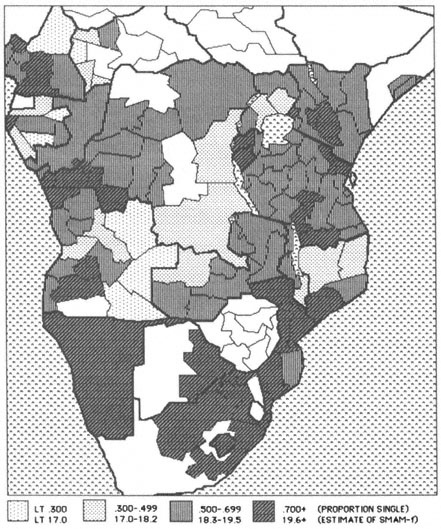
The first issues to be discussed are the ages at entry into a first union and the corresponding sex differential. The parameters used in map 6.2 are the proportions of single women 15–19 and the singulate mean age at marriage for women (SMAM-f ), which corresponds to this proportion according to the link established in eq. 6. 1. The following geographical pattern emerges:

1. A broad zone characterized by early marriage for women (SMAM values commonly below 18) lies in the western and central savannah and sahel regions, which contrast strikingly with a belt of later ages at marriage (commonly above 18 and often above 19.5) along the Atlantic. This Atlantic belt stretches all the way from Liberia to Namibia and is interrupted only in Gabon and Angola (provided that the data quality in these two countries was adequate in the 1960s). The inland boundary reaches from Monrovia in Liberia to Ilorin in Nigeria (Kwara state) and bends south to the Cameroon highlands, Congo, Bandundu province of Zaire, and Northwest Angola. The area of late female marriage continues with Southwest Angola until it reaches the Cape.

2. Several populations north of the sahelian strip of low female ages at marriage have higher values. This pertains particularly to Saharan nomadic groups who are often related to North African Berbers (for example, Hassania of Mauritania, Twareg).

3. There is a second strip of ages at marriage above age 18 for women covering much of East and South Africa. It contains pockets with SMAM values above 19 in Central Kenya, Rwanda, Burundi, and Northeast Tanzania. These pockets are welded together further south where ages at marriage above 19.5 become the rule in South African ethnic groups. Very recent survey data for the whole of Zimbabwe (1984) yield a SMAM value of just over 18, so that most of the blank area on map 6.2 for this country has presumably kept the Zambian pattern and has not yet adopted the South African system of very late marriage. Pockets of early marriage, that is, below 18, are also present in East Africa, for instance in Central Uganda, South Malawi, and North Mozambique.

4. It is not entirely clear whether the region of early female marriage in the western and central sahel still spreads along a north-south axis into Central Africa, as it did in the past. The data for Central, South, and East Zaire are old (that is, from 1955) and if a general trend toward later marriage has occurred, the contrast with West Zaire (data of 1975), Tanzania (1979), and Zambia (1969) may be artificial. Ages at marriage, however, in the Central African Republic, East Angola, and Northwest Zambia recorded in the 1960s further support the probable historical existence of such a central African area with SMAM values commonly lower than 18 years. If, on the other hand, mean ages at marriage have risen in central Africa, a general evolution towards a more simple dichotomy is probably underway, contrasting continued early marriage for women in the largely Islamized western and central savannah and sahel with mean ages at marriage over 18 for the rest of Africa.

Map 6.1a .
Statistical Areas, West Africa (see Key 6.1)

Map 6.1b .
Statistical Areas, East Africa (see Key 6.1)

5. Sudan, Ethiopia, and Somalia have been omitted from the discussion until now. Fragmentary evidence suggests than SMAM values for women were lower than 18 years in the 1960s, but recent surveys in Somalia and North Sudan (WFS) suggest a substantial rise. For North Sudan it is highly likely that this rise can, at least partially, be attributed to marital status–related age misstatement (cf. figure 6.1). Hence it is too early to come up with a definitive judgment regarding a recent trend.

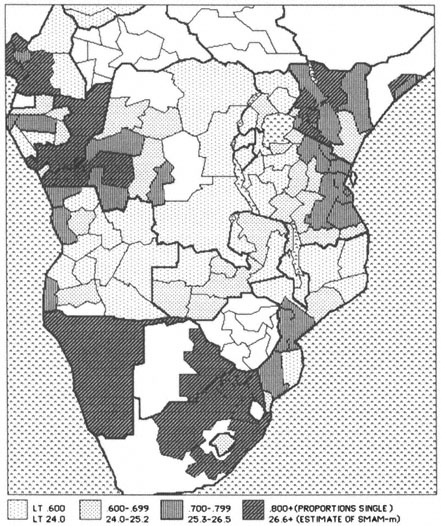
The map with the male proportion single 20–24 or male SMAM values based on these proportions differs greatly from the map with the comparable female values (see maps 6.2 and 6.3). There is no western sahelian pattern of early marriage for men and the "Atlantic crescent" no longer provides a continuous string of late age at marriage (that is, above 25). The Central African north-south strip of early marriage for males (that is, below 25) extends well into East Africa, even if data from the late 1970s are used. The only major similarity with the distribution of female marital behavior is an overall pattern of late marriage for both sexes in South Africa, Botswana, and Namibia. The proportions single for the two sexes can be contrasted by means of the SMAM difference computed via equations 6.1 and 6.2. As indicated above, the lowest difference in husband-wife ages at first marriage is 3 years and the highest 11. Taking 7 years as a cutoff point, one can readily see on map 6.4 that the largest husband-wife differences are especially concentrated in West Africa. Differences in excess of 9 years (omitting Sudan, Ethiopia, and Somalia) only exist in the western Islamized areas, such as in Senegal, Guinea, and Central Burkina Faso. In East and South Africa, husband-wife age differences at first marriages between 7 and 9 years are only found in North Kenya and the Kenyan Rift Valley, and among the Tswana, Ndebele, and Venda ethnic groups of South Africa. Age differences in excess of 7 years are hence the rule in West Africa and the exception elsewhere. SMAM values computed on the basis of the full age schedule of proportions never-married or ratios of proportions single (RPS ) convey a similar picture.

The geographic distribution of SMAM differences is obviously related to the pattern of polygyny. The comparison of map 6.4 showing the SMAM differences between the sexes with either map 6.5, showing the proportion of women currently married to a polygynist (f ), or map 6.6, with polygyny ratios (M ), testifies to this effect. The Atlantic polygyny zone stretches far inland and incorporates all climatic and cultural zones of West Africa. The high polygyny zone extends further south to Angola. The only Atlantic areas with less than 40 percent of married women in polygynous unions and polygyny ratios below 1.3 are found in Southeast Ivory Coast and Southwest Ghana (that is, in matrilineal Akan ethnic groups) and in the border regions of Southeast Nigeria and Southwest Cameroon. Finally, sahelian nomads

Map 6.2a .
Proportion Single Women Aged 15–19 and Approximate Values of the Female
Singulate Mean Age at First Marriage (SMAM-f); Latest Available Data

and Berber groups have a very low incidence of polygyny and do not fit the sub-Saharan pattern at all (see, for instance, Randall on the Tamasheq Twareg, 1984, and the WFS-results for the Hassania of Mauritania).

In general, the incidence of polygyny in Central, Eastern, and Southern Africa is much lower than in the Atlantic zone and the western sahel. There are, however, a few exceptions. Polygyny ratios above 1.20 or percentages of women married to polygynists in excess of 30 (still modest by West African standards) are found in West Kenya, Central Tanzania, East Zambia, North Malawi, and North Mozambique, forming an East African polygyny ridge that stretches south from Kisumu on Lake Victoria to the Tete province of Mozambique. In places along the coast of the Indian ocean values of M larger than 1.20 or f larger than 30 percent are also found: for example, in the Kenyan Coast province; the Tanzanian districts of Tanga, Lindi, Mtwara, and Ruvuma; the Mozambique province of Manica-Sofala; and among the coastal Nguni (Zulu) of South Africa.

The polygyny multiplier KL (that is, the ratio of proportions currently married of both sexes) and its major component L (that is, the ratio of proportions ever-married women and men) change the information given by the polygyny ratio M and the proportion of women in polygynous unions f to a considerable extent. One may recall from the previous section that KL is not positively affected by the adult sex ratio F/M. Consequently, areas with high values of M and f, but also with a substantial surplus of adult women, no

Map 6.2b .
Proportion Single Women Aged 15–19 and Approximate Values of the Female
Singulate Mean Age at First Marriage (SMAM-f); Latest Available Data

Map 6.3a .
Proportion Single Men Aged 20–24 and Approximate Values of the Male
Singulate Mean Age at First Marriage (SMAM-m); Latest Available Data

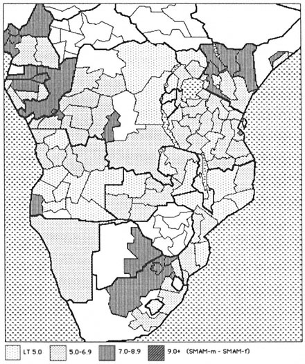
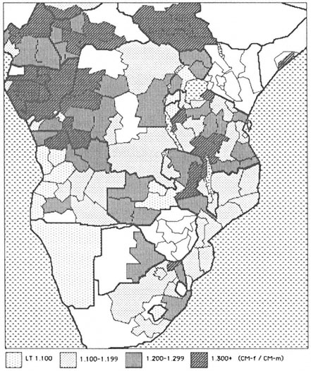
longer show up with dark shadings in map 6.7 presenting the polygyny multipliers. This results in the total disappearance of the East African polygyny ridge. With very few exceptions, polygyny multipliers do not exceed 1.20 in Central, East, and South Africa.

The picture for West African polygyny, measured by M or f, undergoes similar modifications if the polygyny multiplier KL is used. It should be noted, in passing, that KL values larger than 1.20 are the rule in West Africa, which makes the East-West contrast even sharper in map 6.7 than in the preceding polygyny maps. The map with polygyny multipliers closely resembles the map with SMAM differences (map 6.4). This is reflected in correlation coefficients: M and the sex difference in SMAM have a coefficient of 0.42, whereas KL and the SMAM -difference have a coefficient of 0.60.

Several of the West African areas that had been singled out for their relatively low incidence of polygyny (that is, Akan groups, Nigerian-Cameroon border area), no longer stand out once the polygyny multiplier is used. The KL values act to smooth out the data and present a more even picture.

Map 6.7 contains, however, one major exception: several regions in southern Nigeria with high values of M and f, have low values of KL. It is suspected that this exception is artificial: Nigerian sex ratios were obtained in the WFS household survey, whereas sex ratios for other countries are derived from censuses or much larger surveys. Given the small samples by state in the Nigerian WFS and the focus of attention on the fertility-oriented indi-

Map 6.3b .
Proportion Single Men Aged 20–24 and Approximate Values of the Male
Singulate Mean Age at First Marriage (SMAM-m); Latest Available Data

Map 6.4a .
Husband–Wife Age Difference at First Marriage; Latest Available Data

vidual questionnaire, an accurate recording of men in the household or elsewhere was less likely. An idea of the size of the error can be obtained from comparing the adult sex ratios in Cameroon as measured through the Cameroon WFS of 1978 and the census of 1979. This comparison is illustrated in table 6.4. The areas are ranked by surplus of women, from high to low, and the ratio between the two series indicates the relative magnitude of the deviation. These Cameroon data indicate that the ranking is similar for both sources, but that deviations by area can be as high as 16 percent. The largest

Map 6.4b .
Husband–Wife Age Difference at First Marriage: Latest Available Data

Map 6.5a .
Proportion of Currently Married Women Aged 15+ in Polygynous Unions

discrepancies are found in areas experiencing either considerable emigration (Western Highlands) or immigration (Southwest, Littoral). The WFS systematically produces a higher surplus of women, which is not surprising given that the main purpose of the household questionnaire was the identification of women of childbearing age. In Cameroon, greater care was taken to collect more detailed household-level information than in the other countries participating in the WFS, and it can be assumed that the WFS adult sex ratios for Cameroon are better than elsewhere. Morah (1985) compared the age specific sex ratios in the Nigerian WFS household data with those of the 1963 census and found a much larger excess of females in the age range from 15 to 60 in the national WFS-data set. In the age group 20–24, there were for instance 155 women per 100 men and in the age group 25–29 152 women. This anomalous pattern was less marked in the 1963 census with 119 and 114 women respectively. In view of this, it is entirely plausible to assume that the low KL values for southern Nigeria are the result of highly inflated sex ratios. Ogun state, for instance, has an adult sex-ratio for the entire population over 15 of 160 women per 100 men. The general conclusion is therefore that WFS data can be used to estimate values of f , but not for measuring M , KL , and sex ratios.

The issue of sex-ratio imbalances warrants further attention. There are two major sources of such imbalances: (1) measurement error as suspected, for instance, in the WFS household data, and (2) sex and marital status

Map 6.5b .
Proportion of Currently Married Women Aged 15+ in Polygynous Unions

Map 6.6a .
Polygyny Ratio; Latest Available Data

selective migration. Interaction between these two sources of variation may also occur. For instance, husbands who have migrated may accurately report the number of their wives but not specify their location. These women are then assumed to have migrated with them. If the wives are, however, in the area of origin, they risk being counted twice.

Most African migration streams are largely composed of men. The composition by marital status of the male migrants is more variable. The Voltaique migration to the Ivory Coast involves mainly single men, whereas the labor migration in South Africa involves all men. To what extent can the adult sex ratios of map 6.8 be explained in terms of migration? Table 6.5 contrasts the sex ratios of areas that are economically attractive with those of either neighboring zones of labor recruitment or economically disadvantaged areas. It is encouraging to find that the largest contrasts in adult sex ratios within countries are strongly associated with known migration streams and contrasts in regional population growth. Hence, the information in map 6.8 is not predominantly the product of measurement error.

The positive association between the polygyny ratio M and the adult sex ratio F/M (r = +0.50) has been given a specific interpretation in West African populations with a high incidence of polygyny. Capron and Kohler (1975) suggest that polygyny and male emigration are mutually reinforcing. This thesis is supported by data from the Mossi of Burkina Faso. The absence of young Mossi men gave the older, wealthier men, who remained at home, more opportunities for "monopolizing" the pool of available women.

Map 6.6b .
Polygyny Ratio; Latest Available Data

Map 6.7a .
Ratio of Proportions Currently Married 15+ or
Polygyny Multipliers; Latest Available Data

This resulted in bridewealth inflation and enhanced polygyny, consequently pushing more young Mossi to emigrate to the Ivory Coast in pursuit of means for financing the acquisition of a first wife. Strong gerontocratic control, polygyny with early marriage for girls, emigration of single men, and subsequent male marriage postponement formed the basic ingredients of this particular nuptiality regime. It is possible to imagine the alternative, the young migrants earning enough independently to compete with the older men in the marriage market. However, independent earnings are so strongly connected with a period of exile that even if the earnings are large enough, time abroad is still being lost, thereby resulting in a longer period of marriage postponement.

It would be dangerous to interpret the positive association between the polygyny ratio (M ) and the adult sex ratio exclusively in these terms. Alternatively, a surplus of married women is likely to be found wherever there is a surplus of women resulting from emigration of married males. Then, M is simply statistically contaminated by the adult sex ratio even in areas with much less polygyny.

The information presented in the various maps was compared and systematized through classic statistical procedures. First of all, it was considered fruitful to reduce the nine original indicators into a smaller number. This was done with a minimal loss of information by means of factor analysis. The underlying factors of the original set of indicators were defined in such a way

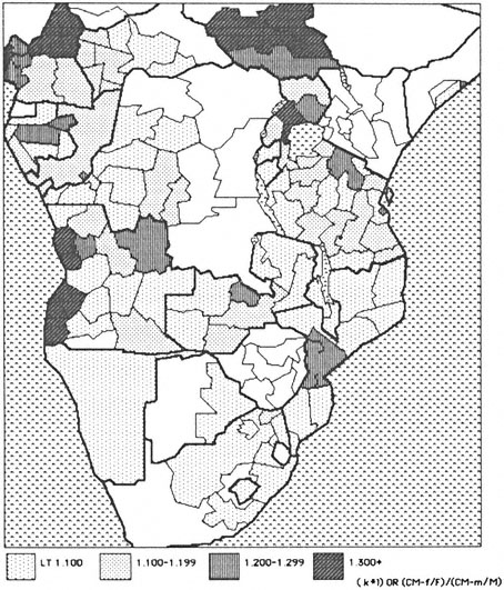
Map 6.7b .
Ratio of Proportions Currently Married 15+ or
Polygyny Multipliers; Latest Available Data

Map 6.8a .
Sex Ratios of Population Aged 15+ (Females/Males); Latest Available Data

that they bore no relation to each other (orthogonal factor extraction). In this instance, seven of the nine original indicators were used: the remaining two measure the differences in ages at marriage for men and women (SMAM difference and RPS ) and they are derived algebraically from the indicators of age at first marriage belonging to the first set. It was therefore statistically impossible to introduce them simultaneously with their components. Correlation coefficients of the SMAM difference and RPS with the factors defined by the first seven indicators were obtained subsequent to the factor extraction, and these values are reported in the bottom section of table 6.6.

The factor analysis results point to the existence of three major factors that jointly explain almost 80 percent of the original variance. Factor identification can be achieved through the single best indicators:

1. Factor 1 correlates strongly with the two measures of polygyny M and f . As expected, the correlations with the measures of the age gap at first marriage (SMAM difference and RPS ) are substantial. Those with the proportions single and with the adult sex ratio are equally logical in view of our previous discussion.

2. Factor 2 is identified by the adult sex ratio F/M. But, also a substantial negative association is found between L, that is, the main component of the polygyny multiplier, and factor 2. Moreover, this correlation is stronger than the one between L and the polygyny factor, which may seem surprising. At this point, it is necessary to recall that migration of

Map 6.8b .
Sex Ratios of Population Aged 15+ (Female/Males); Latest Available Data

TABLE 6.6  Major Underlying Dimensions of Sub-Saharan Nuptiality Indicators; Results from Factor Analysis   NOTE: Principle factoring (PA2) is used with VARIMAX and orthogonal rotation of factor axes.

single men distorts both the sex ratio and L in opposite directions: emigration of single men obviously raises the overall surplus of women and it increases the proportion of ever-married men, which is the denominator of L. Factor 2 can then be interpreted as carrying the effect of sex and marital status–differentiated migration. Equally noteworthy is the negative association between factor 2 and the SMAM difference (r = –0.52). If the effect of polygyny is factored out, a typical migration and marriage market feature emerges: for the overrepresented sex in an area, the proportion single below age 20 for women or 25 for men tends to increase and for the underrepresented sex it tends to decrease. In the instance of a female surplus, the corresponding SMAM values for women rise, whereas they fall for men. The correlation coefficients between factor 2 and the SMAM difference or RPS are entirely in line with this. It should, however, be stressed that proportions single and SMAM values are no longer valid indicators of ages at marriage in populations that are subject to substantial sex and marital status selective migration. Factor 2 correctly documents the concentration of young single

men in immigration areas, but one should be cautious in interpreting this as indicative of late marriage for men.

3. Factor 3 is identified by the two indicators of ages at first marriage. Both factor coefficients are positive: if polygyny and sex ratios are factored out, a geographical pattern remains that describes the overall timing of marriage for both sexes jointly.

4. The only indicator with low factor coefficients throughout is K. Evidently, the geography of the sex differences in proportions currently widowed and divorced constitutes a dimension on its own and accounts for a portion of the variance not explained by the three previous factors.

The ratio of proportions currently married K needs further discussion. It may be recalled that high values of K indicate a small surplus of the proportion widowed and divorced women in relation to the proportion widowed and divorced men. This is typically produced by a rapid relative pace of remarriage for women. K is furthermore less affected by sex-ratio distortions (r = –0.14), in contrast to L, the other component of the polygyny multiplier. Areas with a small relative surplus of proportions widows and divorcées are commonly found north of the line running from Douala in Cameroon to Cabo Delgado in Mozambique (K larger than 0.90), and areas with the smallest surplus (that is, K larger than 0.95) are almost exclusively found in West Africa. Such fast remarriage is consistent with high levels of polygyny in West Africa. On the other hand, large relative surpluses of widows and divorcées, that is, low values of K , are common in Zambia, Namibia, Lesotho, South Mozambique, and Botswana. This is equally consistent with low levels of polygyny and the presence of female-headed households instead. Mauritania has also low levels of K, fitting the low level of polygyny among its Arab population.

But there has been an enigmatic finding in the dominance of low levels of K in the area made up by South Cameroon, Gabon, Congo, and West Zaire, which is neither characterized by the existence of female-headed households, nor by low polygyny. In fact, it is the existence of this zone which prevents K from falling into a closer relationship with the other indicators of nuptiality and polygyny; further, this zone is responsible for the low factor coefficients of K reported in table 6.6.

Factor analysis has enabled the basic dimensions underlying the various nuptiality and polygyny indicators to be teased out. A few determinants were also collected for the regions and their effects were examined by multiple regression. The most important covariate is female literacy. Where actual measurement of illiteracy was missing it was measured as the proportion of women without formal schooling, in both cases for women 15–19. The information was limited to the youngest age group, primarily because most

first marriages for women occur before age 20. The proportion of illiterate women 15–19 also reflects the general level of illiteracy in the population and serves to distinguish those populations that have undergone a boost in female schooling and those which have not. The other covariates are the logarithm of population density and year of observation. Population density indicates the presence of urban concentrations, normally associated with higher ages at marriage for women and less polygyny. It also captures the presence of population concentration in rural areas which, often for geographic and climatic reasons, have had high population densities in the past (for example, Rwanda, Burundu, Central Kenyan Highlands, areas around Lake Victoria, and so forth). Population pressure in these rural areas is often considerable, and it is conjectured that this could result in the postponement of marriage. The year of observation is added to examine the effect of variation in the periods of observation.

The first set of dependent variables is made up of the indices of age at first marriage and the sex differences in these ages. The regression results are shown in table 6.7 in the form of beta-coefficients (that is, standardized regression coefficients). The zero-order correlations are provided for comparison. The results for the proportion of women single 15–19 and the ratio of proportions single (RPS ) are of necessity similar, given that RPS is influenced more by the proportion of women single 15–19 than the SMAM difference. The strongest determinant was female illiteracy, which exhibited the classic inverse relationship with proportions single women 15–19 and RPS: areas with high female illiteracy have earlier marriage for girls than areas with better schooling. This not only supports butjustifies the extension of the findings made in chapters 2 and 3 to the rest of sub-Saharan Africa.

The results for the variable "year of observation" were also significant: areas contributing recent observations tend to have later female marriage and higher RPS -values. But this should not be used as evidence of a rising trend in female age at marriage. Areas that are more developed socioeconomically also tend to have more recent data sources, while other, less developed areas are often described by a single, older source (such as Central African Republic, Chad, Bukina Faso, Mali, Guinea, South Sudan, East and North Zaire).

Male age at marriage and the SMAM difference were less affected by female literacy, but more so by polygyny. This reflects the fact that high male ages at marriage and the concomitant large age gap between spouses are almost exclusive to the West African polygyny belt. The extension of the study area beyond West Africa alters a finding of chapter 2, where a closer relationship between polygyny and female age at marriage was found. Hence, there is a plurality of factors associated with low ages at marriage for women and a more dominant single factor, that is, polygyny, associated with late marriage for men.

TABLE 6.7  Effects of Selected Variables on Measures of Age at First Marriage and Age Difference at First Marriage Dependent Variable   Zero-Order Correlations and Beta-Coefficients     Proportion Women 15–19 Illiterate Sex Ratio F/M Proportion Married Women in Polygynous Union Log of Population Density Year of Observation R2 R Proportion women 15–19 single               zero-order –.62 +.05 –.31 +.20 +.41     = .57  s= .20  beta –.63* +.03 +.06 –.07 +.39* .52 .72 Proportion men 20–24 single                 zero-order –.08 –.12 +.28 +.32 +.27     =.69 s =.13  beta –.42* –.28* +.60* +.21 +.01 .30 .54 Age difference at first Mariage                 zero-order +.40 –.21 +.53 +.19 –.01     =6.5 s = 1.6  beta +.04 –.36* +.59* +.04 –.06 .42 .65 Ratio proportion single women 15–19  to proportion single men 20–24 (RPS)                 zero-order –.62 +.17 –.49 –.01 +.27     = .83 s = .27 beta –.44* +.23* –.27* –.11 +.30* .53 .73 *Denotes significance at .05 level; N varies from 104 to 201.

Imbalances in adult sex ratios also have an impact on the proportion of single men 20–24 and the SMAM difference. A large surplus of women tends to lower male ages at marriage and the age difference between the spouses (cf. factor analysis results above). Population density, however, fails to produce significant results: the small positive zero-order correlations with both proportions single were as expected, but they vanish once literacy and polygyny are introduced.

The second set of dependent variables includes polygyny measures and the components of the polygyny multiplier. The regression results are shown in table 6.8. Attention is again directed to the effect of female schooling in view of the Westernization thesis of Goode and Caldwell. Despite the introduction of the proportion of women single 15–19, which is itself influenced by literacy, a strong positive and direct effect of female illiteracy on the polygyny indicators M and f is found. Areas with more literacy tend to have less polygyny, not only because women marry later in such areas, but also because of the direct polygyny-reducing effect of higher literacy. This is in line with Goode's hypothesis, but also consistent with Boserup's thesis that polygyny is a form of appropriation of female productive capacity in societies with traditional, low-technology agriculture. Given a negative relationship between subsistence agriculture and female education, one can indeed expect a negative association between female literacy and polygyny. The relationship between female illiteracy and the polygyny multiplier is smaller, but still in the direction suggested by Goode.

It is interesting to note the finding that higher female illiteracy is associated with higher K values, or with a smaller relative excess of widows and divorcées and faster remarriage of women. In other words, low literacy is associated with the minimization of the loss of reproductive capacity through celibacy, divorce, and widowhood.

The coefficients of proportions single are all in the expected direction and do not warrant further attention. Neither do the coefficients of the sex ratio since they show once more that the two types of polygyny measures (M and f versus KL and L ) are distorted in opposite directions. The coefficients of "year of observation" are nonsignificant throughout, and the effects of density on f and K essentially measure the East-West contrast.

The regional information for the components of the sub-Saharan nuptiality regimes can be summarized by the following:

1. With the exception of Arabs and Berbers, West African populations have considerably higher levels of polygyny, larger age gaps between spouses and faster remarriage then Central, East, and especially South African ones.

2. Islamized populations in West Africa have particularly early ages at marriage for women. This is partially due to high levels of female illiteracy. Non-Islamized populations of the region often reach similar

TABLE 6.8  Effects of Selected Variables on Measures of Polygyny and Components of the Polygyny Multiplier Dependent Variable Zero-Order Correlations and Beta-Coefficients   Proportion Women Single, 15–19 Proportion Men Single, 20–24 Proportion Women Illiterate, 15–19 Sex Ratio F/M Log of Population Density Year of Observation R2 R Proportion of married women in polygynous unions (f)   zero-order –.31 +.28 +.57 +.27 +.18 –.02     =.40   s = .14 beta –.20 +.42* +.54* +.40* +.28* –.09 .65 .80 Polygyny ratio (M)                   zero-order –.33 +.14 +.49 +.50 –.05 –.10     =1.28 s = .17 beta –.31* +.36* +.59* +.37* +.07 –.01 .63 .79 Polygyny multiplier (KL)                   zero-order –.34 +.32 +.52 –.54 +.13 +.05     =1.16 s =.16 beta –.30* +.30* +.36* –.44* +.05 +.01 .60 .77 Ratio of proportion ever-married (L)                   zero-order –.23 +.36 +.38 –.52 +.04 +.05     = 1.29 s = .15 beta –.35* +.50* +.16 –.45* –.15 +.09 .56 .75 Ratio of proportion currently married (K )                   zero-order –.25 +.01 +.39 –.14 +.24 +.01     =1.90 s =.07 beta +.02 –.06 +.44* –.07 +.36* –.10 .26 .51 * Denotes significance at .05 level; N varies from 104 to 201.

polygyny levels, but these are based on higher ages at marriage for women.

3. First marriage for men tends to be early in East Africa, which is in line with the more modest levels of polygyny. But male ages at marriage are particularly high in southern Africa, despite low polygyny levels. This undoubtedly reflects the disruption of traditional nuptiality patterns by vast male labor migration and the concomitant social and economic constraints on household formation typical for this region (see also chapter 8).

4. Male emigration is associated with enhanced polygyny in West Africa, but not in Southern Africa, where the response to it has been the emergence of female-headed households.

5. Apart from polygyny, the regional distribution of proportions single is also affected by migration and sex ratio distortions, largely because of the sex and marital status specificity of migration streams. Male emigration and the resultant surplus of women usually lead to enhanced proportions single among women 15–19 in the sending area. Conversely, in the receiving areas, males form the overrepresented sex with large accumulations of single males aged 20–34. SMAM values for regions experiencing heavy migration, in or out, do not reflect the real ages at first marriage of their individuals because of the violation of the stationarity hypothesis underlying the calculation of SMAM.

6. The cross-sectional associations of female literacy with female ages at marriage and polygyny are impressive and in the direction expected by Goode's thesis. They are, however, not directly interpretable as supporting Goode's proposition, which postulates, first, a causal link, and second, a general trend towards later marriage and less polygyny. There are "common causes" at work in the cross-section used so far, and these simultaneously affect female literacy, female age at marriage, and polygyny. For instance, simple technology in agriculture (that it, hoe agriculture) with heavy involvement of women is also correlated with low female literacy, early marriage, and high levels of polygyny (cf. Boserup's thesis). Islamization too depresses female literacy and enhances early female marriage as a result of the tighter control over women and partner selection (cf. Goody's thesis). The causal interpretation of the cross-sectional correlations between female literacy and the components of the nuptiality regime is, therefore, partially spurious since other social organizational variables are involved. Without statistical controls for these variables, the cross-sectional results are of limited use in inferring trends towards later marriage and less polygyny. What happens if such statistical controls are provided and if the traditional patterns of social organization are allowed to play their role? Before answering this question, a reformatting of the data according to ethnicity is required. This is taken up in the next section.