Measurement Problems and the Definition of Indicators

The broad definition of marriage used in most censuses and surveys fits the needs of demographers since they are only interested in whether or not an

individual is in a regular sexual union. Sometimes further distinctions are made between different types of unions: legal, traditional, consensual, and so forth. Occasionally census reports contain tabulations of the frequency of the different types of unions. The broad definition found in censuses is in fact a reflection of the situation in reality: different ethnic groups and religious faiths proscribe different forms of marriage. In fact, the legal codes of countries often specify different regulations for different union types. In Tanzania, for instance, Muslim and traditional marriage are presumed to be potentially polygynous, while others are not. But in fact the form of marriage can be changed by a mutal declaration of the spouses (Marriage Act of 1971), so that in practice all marriages are potentially polygynous.

Although such a broad definition of marriage covers most sexual unions, there still remains a problem in comparing the different types of unions internationally because of variations in local legislation and interpretation. A form of union often excluded is that of a visiting relationship. These "outside wives" or "deuxièmes bureaux" are commonly found in urban areas and are presumably classified as consensual unions (marriages d'amitié) or single. Whereas from the demographer's point of view these women are effectively married in that they are in a regular sexual union and often have children, from the anthropological point of view they are not. Marriage legitimates and thereby institutes social inclusion of sexuality and fertility. From this point of view "outside wives" are more akin to concubines than to women in a polygynous union since they are external and often illicit. But demographically they are of significance as an alternative mode of reproduction in societies undergoing socioeconomic change. As pointed out before, in many cases these women will be lost between the different marital status categories. Some surveys, however, and the WFS in particular, include a final question referring to the existence of any partner, which allows "single" women to admit to having a partner and being recorded as being in a union.

More serious than the problem of definitions is the undisputed tendency of the ages of women to shift across the 5-year age boundaries according to marital status. Married women younger than 15 tend to be recorded as 15–19 years old, and single women older than 20 tend to be dropped down into the same age group. Similarly, married women 15–19 may be pushed into the 20–24 category when age-heaping is particularly prevalent (rounding to 20). This practice can be severely aggravated if literacy levels are low and if the interviewer uses marital status or parity to determine a woman's age. In 1955, Romaniuk (1968) found in Zaire that there was an evident correlation between the regional index of age misreporting for women aged 10–14 and 15–19 and the estimated mean age at marriage (r = 0.74 and 0.48 respectively). This was attributed to age overstatement by married and postpubescent girls and to the fact that interviewers had been explicity instructed to estimate ages on the basis of marital status. Interestingly, Romaniuk also found

a similar phenomenon for men, but solely for the age group 15–19, despite the lack of such instructions. It can be assumed that in practice interviewers used the same techniques for age estimation for men and women alike, but given the concentration of marriage for women in just one age group (15–19), interviewers could assign ages more easily on the basis of marital status for women than for men.

Since the degree of literacy among young women in non-Muslim areas was greatly enhanced in the 1960s and 1970s, it is plausible to assume that the quality of the age data has correspondingly improved. In sub-Saharan Africa, furthermore, the overall regional variation in the proportions of single women and men is so great that the relative error involved in interregional comparison is moderate. The quality of the age data collected after 1970 is probably more reliable, but the unevenness over time creates major problems in estimating trends. Indeed, the analysis of trends is very susceptible to bias given the differential degree of distortion of the two or three successive estimates used. The cross-sectional analyses based on spatial and ethnic patterns may, therefore, prove to be more accurate than the trend analyses.

A third problem that arises in survey data analysis is the increasing unreliability of retrospectively reported ages at first marriage with the advancing age and decreasing literacy of respondents. There is a tendency to round ages to multiples of 5, which is accompanied by an upward shift to 20 and 25. Van de Walle's golden rule is to never trust retrospectively reported ages at marriage for women who cannot specify their age or year of birth. This rule has its obvious value and the estimation of cohort changes in ages at marriage should consequently be discouraged if the information stems from such retrospectively reported figures obtained in a single survey. Despite this, cohort comparisons are often attempted, notably in WFS reports, with the resulting dubious interpretation of apparent trends.

These points can be documented for the WFS-countries. As displayed in figure 6. 1, quartile and median ages at first marriage often show a U-curve. The left arm of the U is indicative of marital status–related age misstatement. If married women gave or were assigned ages that were too high, the age group 15–19 will contain too many single women. This proportion can be enhanced even more when older single women are subjected to the reverse error. Quartiles and median values for the youngest age group are considerably inflated in such circumstances. The left arm of the U-curve is very pronounced in the WFS data for Northern Sudan, but equally present in the data for Nigeria, Senegal, and Kenya. The right arm of the U tends to rise at about age 30 or 35 and results from an upward rounding of retrospectively reported ages at first marriage. In figure 6.1, the right arm is most obvious in the data for Nigeria and Cameroon. The Ghanaian data have the flattest profile and those for Lesotho (not shown here) are almost free of such distortions. Not surprisingly, the countries with large Muslim and illiterate

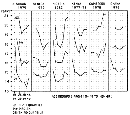
Figure 6.1.
Quartile and Median Ages at First Marriage for Women as Reported
in World Fertility Surveys for Selected Sub-Saharan Countries

populations (Senegal, Northern Sudan, Nigeria) exhibit the strongest U-pattern, whereas those with the most literate populations (Ghana and Lesotho) show relatively minor irregularities.

It is worthwhile to document these points by inspecting the heaping pattern and other indicators of data quality for a particular country. Such a check was carried out on the Kenyan WFS data, which in terms of overall quality were by no means at the poor end of the spectrum. Table 6.2 contains the relevant information. First of all it can be noted that the highest first quartile is for the age group 15–19 and the highest median for 20–24. The lowest median is found in the age group 30–34 and medians and third quartiles rise again thereafter. Hence, the U-shape seems to prevail. The cohort pattern of rounding retrospectively reported ages at marriage now warrants attention. The pattern of rounding to age 10 is highly erratic with over 30 percent of women 35–39 stating this figure, as opposed to only 3 to 8 percent for the youngest and the two oldest cohorts. Child marriage

undoubtedly has declined in Kenya for the more recent cohorts, but the difference between the 35–39 age group and those aboved 40 is entirely implausible. The remarkable attraction to 25 as the age at marriage for those over 30 also suggests dubious data quality. Heaping does not disappear for younger cohorts aged 20–24 and 25–29. They show heaping around a younger age (mainly 20), as expected. The age pattern of self-reported literacy, given in table 6.2, shows a distribution which, in contrast to the increasing levels of schooling, is virtually horizontal. Moreover, the proportions capable of reporting actual dates of birth, first marriage, or even of birth of the last born child (that is, the most recent event) decline with age. In sum, it is rare for more than a quarter of the women to be able to accurately fix a year to an event. In view of this, it seems prudent to follow van de Walle's advice.

Bearing these arguments in mind, it can be concluded that comparisons between regions and ethnic groups based on proportions single by age can be attempted, but that singulate mean ages at marriage for women are likely to be too high for populations with low literacy levels. In fact, the regional variation presented in the next section is likely to be an underevaluation of the true variation. Furthermore, trends inferred from retrospectively reported data have little, if any, validity.

A discussion and presentation of the various indices of nuptiality and polygyny, their definitions and usage, is also necessary. Among the most commonly used indices are:

1. The proportion single among women aged 15–19 and men 20–24. These proportions show the highest regional variance and they are therefore ideal for mapping and illuminating contrasts. But, as shown, they are far from being free of error.

2. Hajnal's singulate mean age at marriage (SMAM ) for both sexes can be produced from the age schedule of the proportions never-married by 5-year age groups. These values are strongly related to the proportions single women 15–19 (PSW ) and men 20–24 (PSM ) respectively, as shown in figures 6.2 and 6.3. For those who prefer the more familiar metric of ages at marriage rather than proportions single, SMAM values can be obtained as:

These conversions are obviously shortcuts, but they illustrate when compared with SMAMs that little is to be gained from the usage of the entire age schedule of proportions never-married in sub-Saharan populations. The only exception to this fit in the entire data file pertains to Saharan nomads or Berber groups (for example, Woodabe

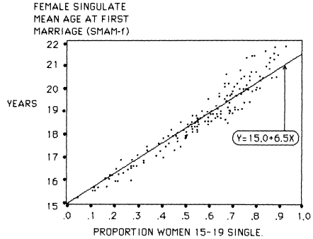
Figure 6.2.
Relationship between Proportions Single Women 15–19 and Female Singulate
Mean Age at Marriage (SMAM-f ).  (Data for Benin, Burkina Faso, Burundi,
Cameroon, Chad, Congo, Ghana, Kenya, Lesotho, Madagascar, Mauritania,
Nigeria, Rwanda, Senegal, Somalia, North Sudan, Tanzania, Togo, West Zaire)

Fulani, Twareg, Hassania) with non-universal marriage among their caste of ex-slaves or servants.

3. The polygyny ratio (M ) the classic index of polygyny, is the ratio of the number of currently married women (CMF ) to the number of currently married men (CMM ). As for all indices, only the population aged 15+ is used here in the computations.

4. Several indices mentioned above can be usefully combined: differences in ages at first union between the sexes can be measured through a ratio of proportions single women 15–19 to the proportion single men 20–24 (that is, the proportions single ratio or RPS ). Alternatively, equations 6.1 and 6.2 can be used to estimate differences between SMAM values for both sexes. Of course, the directly calculated values of SMAM can be used in establishing such differences. The range in SMAM differences is of the order of 3 to 11 years and the age differences between the spouses at first marriage also displays a high degree of regional and ethnic variation.

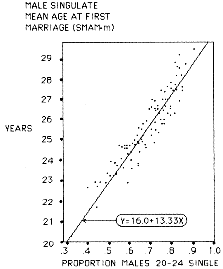
Figure 6.3.
Relationship between Proportions Single Males 20–24 and Male Singulate
Mean Age at Marriage (SMAM-m ).  (Data for Benin, Burkina Faso, Cameroon,
Chad, Congo, Lesotho, Liberia, Madagascar, Mauritania, Rwanda, Senegal,
Somalia, Tanzania, West Zaire)

In addition to these classic indicators, several new ones were employed:

1. The ratio of proportions ever-married (L ), that is the ratio of proportions ever-married women 15+ of all women 15+, to the proportions of ever-married men 15+ of all men 15+:

This ratio is different from the ever-married ratio (EMR), defined as

in the sense that L takes the adult sex-ratio (F/M ) into account. Obviously L = EMR in a population with an adult sex ratio of unity. As shall be shown later on, sex-ratio distortions in the adult population are frequently encountered in sub-Saharan regions, mainly as a result of male migration. It is therefore advisable to have two sets of measures which deal with ratios between numbers and proportions respectively. When differences in ages at first marriage between the sexes are small, both EMR and L approach unity, and when the husband-wife age gap increases, both show a marked surplus of ever-married women. The two measures, however, diverge when sex ratios of adults are no longer balanced.

2. The ratio of proportions currently married (K ) is the ratio of the proportion of currently married women 15+ of ever-married women 15+, to the equivalent proportion for men:

K measures the relative deficit of widowed and divorced men. If the relative surplus of widows or divorcées is preferred, the reciprocal of K is simply used. The values of K are commonly lower than unity since widowhood is more frequent for women (effect of male surmortality, polygyny, and the husband-wife age gap) and since remarriage is generally slower for women than for men. Hence, the lower the value of K , the higher the relative proportion of currently widowed and divorced women, and generally, the slower the relative pace of female remarriage. From the definitions of the classic polygyny ratio M, K and L , it follows that:

or

In other words, the product KL is the common polygyny ratio's counterpart adjusted to the sex ratio, so that KL = M when the adult sex ratio F/M equals unity. Equation 6.6 breaks down the polygyny ratio M into a component L, which reacts to the sex differential in ages at first marriage, a component K, which corresponds to the sex differential in proportions currently widowed and divorced, and the adult sex ratio itself. The product KL can be labeled as the "polygyny multiplier" since it converts the sex-ratio into the classic polygyny ratio. A few further comments with respect to K and L are, how-

ever, warranted. Theoretically, K and L should be independent of the adult sex ratio. This is in practice not so: the polygyny multipliers KL and the adult sex-ratios are jointly influenced by differences with respect to sex– and marital status–related variations in age patterns of mortality, and especially, of migration. Emigration of young single men, for instance, raises the value of the sex ratio by causing a surplus of women, and concomitantly lowers the value of L (that is, emigration of single males increases the proportion of ever-married men in the denominator of L ). Hence, significant inverse correlations between L and the sex-ratio are to be expected. This issue will be returned to during empirical analysis in the next section.

Finally, a number of indices of polygyny, introduced by van de Walle in 1968 and referred to by Goldman and Pebley in the previous chapter, are also used. They are the proportion of polygynists among married men (p ), the average number of wives per polygynist (w ), and the proportion of married females living in a polygynous union (f ). They are related via eq. 6.8:

Censuses and surveys inspired by the French and Belgian traditions of data collection generally provide the data needed for the calculation of p and w , but most data from anglophone countries do not. Parenthetically, the British colonial tradition of demographic data collection paid generally little attention to marital status information despite a rich anthropological legacy in studying marriage, nor has this been rectified during the postcolonial period. Given that only a subset of regions have information on p, w, and f , some complementary information of an equivalent nature was sought. The WFS recorded the number of polygynously married women, but in most instances only for women age 15–49. It was, however, found in the sources for which f is available for the aged group 15+ and 15–49 that the two values were sufficiently similar to be interchangeable. The plot presented in figure 6.4 testifies to this effect. The WFS figures were subsequently added to the series of f without alteration.