Chapter Six—
The Nuptiality Regimes in Sub-Saharan Africa

Ron Lesthaeghe
Georgia Kaufmann
Dominique Meekers

The Issues

In most comparative studies of nuptiality it has been usual to characterize sub-Saharan patterns of marriage as "early and universal." This categorical generalization was shown to be inadequate in the now classic study of van de Walle (1968), which used the then somewhat underweight body of available census and survey data to rigorously examine this accepted opinion. The pioneering work of van de Walle has been taken up and expanded in this chapter.

Although the starting pattern of procreation is not the most significant Malthusian preventive check on population growth in sub-Saharan Africa, it is still worth noting the range of the mean age at first marriage for women, which was found to vary between 15 and 21 years. Such a discrepancy in the average ages of entry into a first sexual union between African populations must have some implications. Interestingly, the Northwest European marriage pattern, first described by Hajnal (1965), of late age at marriage with neolocal, nuclear household formation, exhibits a similar range for mean ages at first marriage among historical European populations. At the very least, the presence of a similar variation in sub-Saharan Africa requires an explanation and it is surprising that there is such a paucity of systematic statistical analysis addressing this problem. At present, most African countries have been covered by at least one census or large-scale survey, and hence it is due time to reopen the African nuptiality file on ethnic and regional variation.

The suspicion that women's ages at first marriage are rising, thereby shortening the overall reproductive age span, provided the second reason for revisiting the subject. The connection between socioeconomic development

or a rise in female literacy and the postponement of marriage with the concomitant increase in the age at first birth has been described for many Third World societies (see Casterline and Trussell, 1980; McCarthy, 1982; McDonald, 1985). The strength and regularity of this positive association in developing countries everywhere is such that the absence of a link is cause to suspect the quality of the data. International evidence, furthermore, indicates that modest rises in female schooling, leading to partial or full primary education only, produces a delay of female entry into regular sexual unions. This trend is not a mere symptom of the practical difficulties of attending school over age 13 while fulfilling a wife's marital duties in the husband's household, but it is the result of changes generated before reaching a marriageable age.

As predicted, it was found that the pattern of rising age at marriage associated with increased levels of female education and literacy was true for sub-Saharan Africa as well. Taking data from several countries, mostly World Fertility Survey participants, it was found for women below 25 that the median age at first marriage rises from 1 year in Benin to over 3 years in Cameroon, Nigeria, and Senegal, as one moves from illiteracy to full primary education (5 to 7 years of schooling). This result, shown in table 6. 1, is not produced by a cohort effect underlying both the rise in age at marriage and the rise of literacy, since the data are derived only from the two youngest age groups.

Since the African cross-sectional pattern by education fits the worldwide experience, and given the increase in female literacy since the 1960s, there is reason for expecting an incipient trend towards overall later female marriage. If this proves to be true, sub-Saharan populations will respond to certain

elements of socioeconomic development, first by a change in nuptiality. This would not constitute an exceptional sequence of events: numerous populations in Latin America and Asia are known to have followed a similar path. In other words, a nuptiality transition has often been a prelude to a subsequent marital fertility transition, and the hypothesis can be advanced that sub-Saharan reproductive regimes have reached this starting point in their adaptation to new conditions. Additional evidence supporting such an outcome has been produced by the analysis of the WFS-data for ethnic groups. From chapter 2 it will be recalled that the spatial distribution of the nuptiality indicator for the youngest age group was very similar to that of literacy and of emerging social stratification by class and was no longer related to the geographic pattern of traditional elements of social organization. By contrast, Goody's variables concerning devolution (inheritance, caste, endogamy) were more successful in predicting the ethnic variation in the age at first marriage for the older women. Obviously, cross-sectional evidence is never an adequate substitute for well-measured trends, but it wets the appetite for further inquiry.

The third reason for returning to the issue of nuptiality is the claim that increased Westernization would lead to a restructuring of the sub-Saharan marriage regimes. In this sense, Westernization is taken to mean the adoption and penetration of Western ideals of conjugal closeness which are spread through the mass media, school textbooks, and Christian doctrine and teaching. Two features of the African nuptiality regime are often suggested to be the most affected by these cultural changes: first of all, increased preference for and tolerance of free partner choice, and second, a weakening in the practice of polygyny.

The hypothesis proposing a shift towards free partner choice is supported by a substantial body of anthropological and sociological research (cf. Dries, 1985, for a bibliography and discussion). Caldwell (1980) has argued that the connection between primary education and changing reproductive behavior can at least be partially accounted for by the spread of Western ideals on partner choice through education and socialization. Indeed, in many parts of Africa literacy is a byproduct of Christian penetration, with its concomitant ideology favoring conjugal closeness. Once a population is literate it is much more open to Western thinking, strongly promoting futher "individualization of marriage."

The literature also draws attention to the disruptive influence of migration, urbanization, and early industrialization (for example, mining) on the traditional social system. The outcome is the possibility of social change, as in new ways of choosing partners in a sexual union. But the weakening of lineage control is perhaps more general. The unilineal system is based on corporate property ownership (land and cattle) and economic interdependence of lineage members. As the lineages lose control over land and economic

independence emerges as a result of integration into the capitalist economy, the freedom of the young lineage members is strengthened as the control of their elders is weakened. This imbalance in social control is further exasperated by the younger members acquiring new skills and abilities (Lesthaeghe, 1980).

The empirical literature describing the evolution of free partner choice not only links it with urban areas, but also testifies to the ambiguity accompanying the change. Even when the choice is individually made, parental consent is still sought so as not to sever the lifeline to the lineage network. It seems that although in the more developed areas of sub-Saharan Africa a change in ways of partner selection is taking place, this has not involved the complete disintegration of lineage control and influence. Despite losing, completely or partially, some of their major rights, kinship groups still fulfil many other duties and functions, which may prove to be crucial to survival in the current economic climate in Africa. At this juncture it is difficult to imagine individuals rejecting the supportive potential of the traditional kinship system completely.

An international study of the various forms of partner selection is beyond the scope of this chapter. The available information is limited to certain areas and the direct measurement of free versus arranged partner selection cannot be attempted through simple demographic or statistical indicators. This is not the case, however, for the second subject of inquiry: polygyny. Western sociologists (such as, Hunter, 1967; Goode, 1970; Gough, 1977) have tended to predict a decline in the incidence of polygyny as part of the universal progression towards a nuclear and conjugal family. The evolutionary notions behind this implicitly view the Western family form as more rational than others. Goode, for example, argues that (1970, p. 188):

It [i.e. polygyny] will, without question, eventually almost completely disappear as a pattern of behaviour. The new legal codes are gradually moving towards its abolition, women will avoid it where they can, and men will not generally be able to afford it.

Not unsurprisingly, Goode was unable to specify a time horizon for this evolution, and any consequent empirical testing of the hypothesis runs the risk of being premature. There are, however, some arguments that are contrary to this evolutionary view. From the functionalist point of view, polygyny has a number of important institutional functions, and as long as there are no viable alternatives to take its place, the existence of the institution is not gravely endangered.

Polygyny, by its nature, causes a large differential marriage age between the sexes, which greatly increases the chance of widowhood for women. But, being functionally coherent, polygyny also provides an efficient remarriage net for widows and divorcées and effectively prevents widowhood for men

(Goody, 1976). Amongst the highly polygynous Konkomba of Ghana and Togo, for instance, instant betrothal is the common practice since all girls and women are already spoken for, resulting in late marriage for men and in frequent widow and fiancée inheritance (Goody, 1973). The institutional alternative to polygyny, in this sense, would be some other social welfare mechanism for the care of the single and elderly. The question remains as to whether such an alternative exists, or is in the making, in response to an initial decrement in the incidence of polygyny.

Since in the lineage system the greatest wealth is sons, polygyny is an insurance against subfecundity or a succession of daughters. Given that large areas of central Africa suffered from high levels of sterility induced by venereal disease, the tendency to increase levels of polygyny there can be seen as a response to subfecundity. In populations where knowledge of contagious diseases and medical treatment is far more disseminated, the logical response would be to curb polygynous practice. In central Africa, however, the logical response to the infecundity problem was simply to marry again. At present, the incidence of venereal disease has declined in this area, probably through the use of antibiotics. Since venereal infection is no longer a major threat, one could argue that the high polygyny levels that came into existence in the past can now be maintained without the risks. This is likely to be an attractive proposition for men over 30 in a region that is largely rural and traditional.

The second point made by Goode in the quotation above concerns the financial ability of men to support a plurality of wives. This argument goes straight to the central issue of polygyny, namely its economic basis. Boserup (1970) was among the first to systematically relate the practice of polygyny to the economic relations of production. Goody (1973, 1976) clearly demonstrates the existence of relationships between hoe-culture and polygyny, and plough-culture and monogamy. Traditionally polygyny was a response to the high productive and reproductive value of women in societies with low levels of agricultural technology and high female participation in cultivation (cf. chapter 1). In many parts of Africa women have continued to be prime economic assets, especially in the agricultural sector. In West Africa, women have a major additional involvement in trade. They continue to generate substantial independent incomes, contributing to household and child care expenses (Schwimmer, 1979). With the current practice of men migrating to the cities leaving their wives in the fields, it is difficult to envisage a radical change in this division of labor. Finally, Clignet (1975) noted how it is the newly arrived migrants who do not practice polygyny (nor would they as young men if they remained at home) and that with time and success, the more established city dwellers return to polygyny or an urban variant thereof (for example, "outside wives"). In East Africa women do more agricultural work, but the men's pastoral activity is seen as more significant. Women in

these predominantly patrilineal societies are valued primarily as producers of sons. Nevertheless, the impact of a monetary income can, as expected by Goode, greatly affect the marital pattern. In Botswana as a result of adapting pastoralism to cattle trading, the relative contribution of women has seriously diminished, and women have been so excluded from the new economic system that not only has polygyny fallen, but marriage itself has gone into decline (Kuper, 1985). To sum up, polygyny can be advantageous to both sexes: men can accrue power and prestige: women gain support, solidarity with cowives, help with child care, and relief from sexual duties. It is probably a more powerful and viable institution than Goode envisaged.

Legal abolition, female education, and Christian conversion have been cited as major forces countering polygyny. In the Ivory Coast, polygyny was legally abolished in 1964, which has done nothing to stop it. Several ethnic groups in the Ivory Coast have been maintaining some of the highest levels of polygyny in Africa. The data on education do show, however, that polygyny declines with increased schooling. Whether this has to do with female choice or other structural factors is debatable: for instance, how capable is a woman with A-levels of farming? The effect of Christianity on polygyny is ambiguous. The Catholic church, in particular, has been waging war against plural marriages throughout its missionary history. The result is either a lax interpretation of official doctrine or its total disregard because of its impracticability. Syncretic churches and Islam have absorbed polygyny and have consequently fared well in terms of recruitment. Hence, the incidence of polygyny may vary substantially by religious denomination, but this should be viewed against the backdrop of selectivity of recruitment. Only in the rare instances where the Catholic church has no major competitors and has a close historical alliance with the state, as in Rwanda, is an effect to be expected.

The immediate concerns of this chapter are the verification and measurement of facts. In the light of this discussion, a realistic research agenda offers the following possibilities:

1. The construction of a nuptiality file and a polygyny file based on census and survey information

2. The study of interregional and interethnic variations for teasing out the sources of this variation

3. The measurement of trends, whenever possible.

Measurement Problems and the Definition of Indicators

The broad definition of marriage used in most censuses and surveys fits the needs of demographers since they are only interested in whether or not an

individual is in a regular sexual union. Sometimes further distinctions are made between different types of unions: legal, traditional, consensual, and so forth. Occasionally census reports contain tabulations of the frequency of the different types of unions. The broad definition found in censuses is in fact a reflection of the situation in reality: different ethnic groups and religious faiths proscribe different forms of marriage. In fact, the legal codes of countries often specify different regulations for different union types. In Tanzania, for instance, Muslim and traditional marriage are presumed to be potentially polygynous, while others are not. But in fact the form of marriage can be changed by a mutal declaration of the spouses (Marriage Act of 1971), so that in practice all marriages are potentially polygynous.

Although such a broad definition of marriage covers most sexual unions, there still remains a problem in comparing the different types of unions internationally because of variations in local legislation and interpretation. A form of union often excluded is that of a visiting relationship. These "outside wives" or "deuxièmes bureaux" are commonly found in urban areas and are presumably classified as consensual unions (marriages d'amitié) or single. Whereas from the demographer's point of view these women are effectively married in that they are in a regular sexual union and often have children, from the anthropological point of view they are not. Marriage legitimates and thereby institutes social inclusion of sexuality and fertility. From this point of view "outside wives" are more akin to concubines than to women in a polygynous union since they are external and often illicit. But demographically they are of significance as an alternative mode of reproduction in societies undergoing socioeconomic change. As pointed out before, in many cases these women will be lost between the different marital status categories. Some surveys, however, and the WFS in particular, include a final question referring to the existence of any partner, which allows "single" women to admit to having a partner and being recorded as being in a union.

More serious than the problem of definitions is the undisputed tendency of the ages of women to shift across the 5-year age boundaries according to marital status. Married women younger than 15 tend to be recorded as 15–19 years old, and single women older than 20 tend to be dropped down into the same age group. Similarly, married women 15–19 may be pushed into the 20–24 category when age-heaping is particularly prevalent (rounding to 20). This practice can be severely aggravated if literacy levels are low and if the interviewer uses marital status or parity to determine a woman's age. In 1955, Romaniuk (1968) found in Zaire that there was an evident correlation between the regional index of age misreporting for women aged 10–14 and 15–19 and the estimated mean age at marriage (r = 0.74 and 0.48 respectively). This was attributed to age overstatement by married and postpubescent girls and to the fact that interviewers had been explicity instructed to estimate ages on the basis of marital status. Interestingly, Romaniuk also found

a similar phenomenon for men, but solely for the age group 15–19, despite the lack of such instructions. It can be assumed that in practice interviewers used the same techniques for age estimation for men and women alike, but given the concentration of marriage for women in just one age group (15–19), interviewers could assign ages more easily on the basis of marital status for women than for men.

Since the degree of literacy among young women in non-Muslim areas was greatly enhanced in the 1960s and 1970s, it is plausible to assume that the quality of the age data has correspondingly improved. In sub-Saharan Africa, furthermore, the overall regional variation in the proportions of single women and men is so great that the relative error involved in interregional comparison is moderate. The quality of the age data collected after 1970 is probably more reliable, but the unevenness over time creates major problems in estimating trends. Indeed, the analysis of trends is very susceptible to bias given the differential degree of distortion of the two or three successive estimates used. The cross-sectional analyses based on spatial and ethnic patterns may, therefore, prove to be more accurate than the trend analyses.

A third problem that arises in survey data analysis is the increasing unreliability of retrospectively reported ages at first marriage with the advancing age and decreasing literacy of respondents. There is a tendency to round ages to multiples of 5, which is accompanied by an upward shift to 20 and 25. Van de Walle's golden rule is to never trust retrospectively reported ages at marriage for women who cannot specify their age or year of birth. This rule has its obvious value and the estimation of cohort changes in ages at marriage should consequently be discouraged if the information stems from such retrospectively reported figures obtained in a single survey. Despite this, cohort comparisons are often attempted, notably in WFS reports, with the resulting dubious interpretation of apparent trends.

These points can be documented for the WFS-countries. As displayed in figure 6. 1, quartile and median ages at first marriage often show a U-curve. The left arm of the U is indicative of marital status–related age misstatement. If married women gave or were assigned ages that were too high, the age group 15–19 will contain too many single women. This proportion can be enhanced even more when older single women are subjected to the reverse error. Quartiles and median values for the youngest age group are considerably inflated in such circumstances. The left arm of the U-curve is very pronounced in the WFS data for Northern Sudan, but equally present in the data for Nigeria, Senegal, and Kenya. The right arm of the U tends to rise at about age 30 or 35 and results from an upward rounding of retrospectively reported ages at first marriage. In figure 6.1, the right arm is most obvious in the data for Nigeria and Cameroon. The Ghanaian data have the flattest profile and those for Lesotho (not shown here) are almost free of such distortions. Not surprisingly, the countries with large Muslim and illiterate

Figure 6.1.
Quartile and Median Ages at First Marriage for Women as Reported
in World Fertility Surveys for Selected Sub-Saharan Countries

populations (Senegal, Northern Sudan, Nigeria) exhibit the strongest U-pattern, whereas those with the most literate populations (Ghana and Lesotho) show relatively minor irregularities.

It is worthwhile to document these points by inspecting the heaping pattern and other indicators of data quality for a particular country. Such a check was carried out on the Kenyan WFS data, which in terms of overall quality were by no means at the poor end of the spectrum. Table 6.2 contains the relevant information. First of all it can be noted that the highest first quartile is for the age group 15–19 and the highest median for 20–24. The lowest median is found in the age group 30–34 and medians and third quartiles rise again thereafter. Hence, the U-shape seems to prevail. The cohort pattern of rounding retrospectively reported ages at marriage now warrants attention. The pattern of rounding to age 10 is highly erratic with over 30 percent of women 35–39 stating this figure, as opposed to only 3 to 8 percent for the youngest and the two oldest cohorts. Child marriage

undoubtedly has declined in Kenya for the more recent cohorts, but the difference between the 35–39 age group and those aboved 40 is entirely implausible. The remarkable attraction to 25 as the age at marriage for those over 30 also suggests dubious data quality. Heaping does not disappear for younger cohorts aged 20–24 and 25–29. They show heaping around a younger age (mainly 20), as expected. The age pattern of self-reported literacy, given in table 6.2, shows a distribution which, in contrast to the increasing levels of schooling, is virtually horizontal. Moreover, the proportions capable of reporting actual dates of birth, first marriage, or even of birth of the last born child (that is, the most recent event) decline with age. In sum, it is rare for more than a quarter of the women to be able to accurately fix a year to an event. In view of this, it seems prudent to follow van de Walle's advice.

Bearing these arguments in mind, it can be concluded that comparisons between regions and ethnic groups based on proportions single by age can be attempted, but that singulate mean ages at marriage for women are likely to be too high for populations with low literacy levels. In fact, the regional variation presented in the next section is likely to be an underevaluation of the true variation. Furthermore, trends inferred from retrospectively reported data have little, if any, validity.

A discussion and presentation of the various indices of nuptiality and polygyny, their definitions and usage, is also necessary. Among the most commonly used indices are:

1. The proportion single among women aged 15–19 and men 20–24. These proportions show the highest regional variance and they are therefore ideal for mapping and illuminating contrasts. But, as shown, they are far from being free of error.

2. Hajnal's singulate mean age at marriage (SMAM ) for both sexes can be produced from the age schedule of the proportions never-married by 5-year age groups. These values are strongly related to the proportions single women 15–19 (PSW ) and men 20–24 (PSM ) respectively, as shown in figures 6.2 and 6.3. For those who prefer the more familiar metric of ages at marriage rather than proportions single, SMAM values can be obtained as:

These conversions are obviously shortcuts, but they illustrate when compared with SMAMs that little is to be gained from the usage of the entire age schedule of proportions never-married in sub-Saharan populations. The only exception to this fit in the entire data file pertains to Saharan nomads or Berber groups (for example, Woodabe

Figure 6.2.
Relationship between Proportions Single Women 15–19 and Female Singulate
Mean Age at Marriage (SMAM-f ).  (Data for Benin, Burkina Faso, Burundi,
Cameroon, Chad, Congo, Ghana, Kenya, Lesotho, Madagascar, Mauritania,
Nigeria, Rwanda, Senegal, Somalia, North Sudan, Tanzania, Togo, West Zaire)

Fulani, Twareg, Hassania) with non-universal marriage among their caste of ex-slaves or servants.

3. The polygyny ratio (M ) the classic index of polygyny, is the ratio of the number of currently married women (CMF ) to the number of currently married men (CMM ). As for all indices, only the population aged 15+ is used here in the computations.

4. Several indices mentioned above can be usefully combined: differences in ages at first union between the sexes can be measured through a ratio of proportions single women 15–19 to the proportion single men 20–24 (that is, the proportions single ratio or RPS ). Alternatively, equations 6.1 and 6.2 can be used to estimate differences between SMAM values for both sexes. Of course, the directly calculated values of SMAM can be used in establishing such differences. The range in SMAM differences is of the order of 3 to 11 years and the age differences between the spouses at first marriage also displays a high degree of regional and ethnic variation.

Figure 6.3.
Relationship between Proportions Single Males 20–24 and Male Singulate
Mean Age at Marriage (SMAM-m ).  (Data for Benin, Burkina Faso, Cameroon,
Chad, Congo, Lesotho, Liberia, Madagascar, Mauritania, Rwanda, Senegal,
Somalia, Tanzania, West Zaire)

In addition to these classic indicators, several new ones were employed:

1. The ratio of proportions ever-married (L ), that is the ratio of proportions ever-married women 15+ of all women 15+, to the proportions of ever-married men 15+ of all men 15+:

This ratio is different from the ever-married ratio (EMR), defined as

in the sense that L takes the adult sex-ratio (F/M ) into account. Obviously L = EMR in a population with an adult sex ratio of unity. As shall be shown later on, sex-ratio distortions in the adult population are frequently encountered in sub-Saharan regions, mainly as a result of male migration. It is therefore advisable to have two sets of measures which deal with ratios between numbers and proportions respectively. When differences in ages at first marriage between the sexes are small, both EMR and L approach unity, and when the husband-wife age gap increases, both show a marked surplus of ever-married women. The two measures, however, diverge when sex ratios of adults are no longer balanced.

2. The ratio of proportions currently married (K ) is the ratio of the proportion of currently married women 15+ of ever-married women 15+, to the equivalent proportion for men:

K measures the relative deficit of widowed and divorced men. If the relative surplus of widows or divorcées is preferred, the reciprocal of K is simply used. The values of K are commonly lower than unity since widowhood is more frequent for women (effect of male surmortality, polygyny, and the husband-wife age gap) and since remarriage is generally slower for women than for men. Hence, the lower the value of K , the higher the relative proportion of currently widowed and divorced women, and generally, the slower the relative pace of female remarriage. From the definitions of the classic polygyny ratio M, K and L , it follows that:

or

In other words, the product KL is the common polygyny ratio's counterpart adjusted to the sex ratio, so that KL = M when the adult sex ratio F/M equals unity. Equation 6.6 breaks down the polygyny ratio M into a component L, which reacts to the sex differential in ages at first marriage, a component K, which corresponds to the sex differential in proportions currently widowed and divorced, and the adult sex ratio itself. The product KL can be labeled as the "polygyny multiplier" since it converts the sex-ratio into the classic polygyny ratio. A few further comments with respect to K and L are, how-

ever, warranted. Theoretically, K and L should be independent of the adult sex ratio. This is in practice not so: the polygyny multipliers KL and the adult sex-ratios are jointly influenced by differences with respect to sex– and marital status–related variations in age patterns of mortality, and especially, of migration. Emigration of young single men, for instance, raises the value of the sex ratio by causing a surplus of women, and concomitantly lowers the value of L (that is, emigration of single males increases the proportion of ever-married men in the denominator of L ). Hence, significant inverse correlations between L and the sex-ratio are to be expected. This issue will be returned to during empirical analysis in the next section.

Finally, a number of indices of polygyny, introduced by van de Walle in 1968 and referred to by Goldman and Pebley in the previous chapter, are also used. They are the proportion of polygynists among married men (p ), the average number of wives per polygynist (w ), and the proportion of married females living in a polygynous union (f ). They are related via eq. 6.8:

Censuses and surveys inspired by the French and Belgian traditions of data collection generally provide the data needed for the calculation of p and w , but most data from anglophone countries do not. Parenthetically, the British colonial tradition of demographic data collection paid generally little attention to marital status information despite a rich anthropological legacy in studying marriage, nor has this been rectified during the postcolonial period. Given that only a subset of regions have information on p, w, and f , some complementary information of an equivalent nature was sought. The WFS recorded the number of polygynously married women, but in most instances only for women age 15–49. It was, however, found in the sources for which f is available for the aged group 15+ and 15–49 that the two values were sufficiently similar to be interchangeable. The plot presented in figure 6.4 testifies to this effect. The WFS figures were subsequently added to the series of f without alteration.

Additional Notes on the Formal Demography of Polygyny

In the preceding chapter Goldman and Pebley described the formal demographic conditions that enhance the potential for polygyny and document their findings with data for three countries (Senegal, Cameroon, and Sudan). With access to a much larger data file, it is possible to make some additional remarks, drawing especially on the data from East Africa and the components derived from the breakdown of the polygyny ratio (that is, M = K • L • sex ratio). In setting up a framework for comparison, more attention will be paid to the roles of divorce, widowhood, and remarriage.

Figure 6.4.
Relationship between Proportions Currently Married Women in Polygynous
Unions in Two Age Categories (15–49 versus 15+). (Data for Cameroon,
Central African Republic, Mali, Tanzania, West Zaire)

The age structure is again taken from a stable population. It corresponds with a gross reproduction rate of 3.0 daughters, a Princeton mortality level of 14 West with a life expectancy of 52.5 and 49.6 years for females and males respectively, a growth rate of 2.92 percent, and an adult sex ratio showing a 5 percent surplus of women. This stable age distribution was then combined with various age and sex-specific schedules of entry into first unions and proportions currently widowed and divorced. This parallels the strategy of Goldman and Pebley who used stable age distributions with similar mortality levels, but varying fertility levels and growth rates. The various combinations of age and sex-specific patterns of first marriage are given in table 6.3. The Coale-McNeil (1972) first marriage model, which allows for the reproduction of age-specific proportions ever-married based on three parameters, was used:

• a₀ : the minimum age at which first unions begin to occur

• k : the pace at which first marriage occurs relative to the Coale-McNeil standard

• C : the proportion ultimately marrying.

The value of k gives the tempo of entry into a union by relating the observed time scale to that of the standard. Since the latter approximates to the time scale of marriage in Sweden 1965–1969, African populations

need a fraction of a year to achieve the same increment in proportions ever-married as the increment achieved in 1 year by the standard. Values of k are therefore substantially lower than unity for women. If k = 0.50, the pace of entry into a first union is twice as fast, and if k = 0.33 it is three times as fast as in the standard. As reported in table 6.3, values of a₀ are allowed to vary from 12.0 to 14.0 years for women and from 15.0 to 16.5 for men. The corresponding range for k is 0.33 to 0.50 for women and 0.70 to 0.85 for men. In all instances C was fixed at 0.98, implying nonmarriage for 2 percent only. These parameter values were chosen after having compared the proportions ever-married for the more extreme populations in the data file. Their range can be taken as an adequate representation of the observed spectrum. The corresponding SMAM values are also reported in table 6.3. The three schedules for males and females define the nine possible combinations, A through I, used in further analyses. For each combination, two indices of the sex differential are given: (1) the ratio of proportions single women 15–19 to single men 20–24 (RPS ) and (2) the SMAM diference.

The joint impact of RPS and the differential age and sex patterns of proportions currently widowed and divorced on the polygyny multiplier KL is studied in figure 6.5. Restricting attention to just one pattern of widowhood, divorce, and remarriage, that is, to one of the four planes in figure 6.5, it is clear how strongly the polygyny multiplier is determined by the sex differences in proportions single at young ages. The relationship can be clarified if KL is reviewed in SMAM -difference rather than with RPS. An increment in the SMAM difference by 1 year results, on average, in an increment of approximately 0.06 in the polygyny multiplier KL. This increment is slightly larger than 0.06 if the increments in SMAM differences are small (3 to 4 years) and slightly smaller than 0.06 if the increment in SMAM differences are large (that is, 6 years or more). But, as a rule of thumb, one is not far off if the incremental value of 0.0 6 in KL per year for husband-wife difference in SMAM is maintained throughout. For instance, if two populations with (1) similar proportions currently widowed and divorced men and women, (2) similar stable age distributions with the typically African characteristics specified above, and (3) identical adult sex ratios have a difference in the husband-wife age gap at first marriage of 3 years (that is, populations corresponding with points A and C, D and F, and G and H in figure 6.5), they would show a difference in the polygyny multiplier of 3•0.06 = 0.18 and a difference in the polygyny ratio M of 0.18•sex ratio (F/M ). Two such populations with husband-wife age gaps at first marriage of 3 and 11 years respectively are 8 years apart, and the difference in their KL values would amount to 8 × 0.0 6 approximately. If their adult sex ratio equals 1.050, their polygyny ratios would differ by about 0.50. This contrast defines the real range encountered in sub-Saharan Africa, with polygyny ratios being comprised between 1.10 and 1.60, given balanced sex ratios. The populations A and I in

Figure 6.5.
Relationship between the Ratio of Proportions Single and the
Polygyny Multiplier (L K )  in Different Situations with Respect
to the Incidence of Union Dissolution and Remarriage

figure 6.5 sharing the same conditions with respect to proportions currently widowed and divorced are 7 years apart with respect to their SMAM difference, and one expects a difference in KL of 0.42. The actual difference is 0.38, illustrating that the rule of thumb is not far off the mark even for extreme cases. Furthermore, the four planes of figure 6.5 are virtually parallel, so that this simple rule is applicable to any two populations with identical proportions currently widowed and divorced, irrespective of the level of these proportions.

The matter is different when populations have varying patterns by age and sex of proportions currently widowed and divorced. Restricting the com-

Figure 6.6.
Age Schedules of Percentages Currently Widowed and Divorced
Women and Men in Contrasting West African Populations

parisons to West African populations with similar age patterns but different levels of proportions widowed and divorced, four contrasting combinations were set up. For example, the lowest levels for both sexes in 1976 were found in Senegal and the highest in two regions of Cameroon (see figure 6.6). The four combinations in figure 6.5 are:

• Pattern 1: Low proportions currently widowed and divorced for females (Senegal) and high proportions for men (Cameroon, South-Central). For these conditions to materialize, widows and divorcées would have to remarry fast and predominantly marry men who are already polygynists. For specified values of RPS, the high polygyny multipliers for pattern 1 result mainly from a high average number of wives per polygynist (w ). The death of a polygynist produces many widows who would all be absorbed quickly by other polygynous households. This reflects social conditions governed by gerontocrats and potentates with large harems. As indicated by many observers, "grande polygamie" is not the rule in sub-Saharan Africa and pattern 1 is rather extreme.

• Pattern 2: The Senegalese conditions prevail throughout and remarriage is fast for both sexes. More widowers and divorced men now compete for spouses than in pattern 1 and the incidence of "grande polygamie" diminishes in favor of more monogamously remarried men or more "petite polygamie."

• Pattern 3: The Cameroon West and South-Central conditions prevail with higher proportions widowed and divorced for both sexes; remarriage is slow by West African standards, which lowers the polygyny multiplier.

• Pattern 4: Males have low proportions currently widowed and divorced (Senegal), whereas women have high proportions (Cameroon West). Remarriage for men is obviously fast, but they do not draw as much from the pool of widows and divorcées as in the previous cases. This feature is less typical for West Africa, and pattern 4 constitutes the other extreme.

The effect of these four combinations appears in the form of parallel planes in figure 6.5. The difference in KL is about 0.14 for patterns 1 and 4, whereas that between Senegal and southwestern Cameroon amounts to about 0.08. With balanced sex ratios, it can be taken that West African patterns of divorce, widowhood, and remarriage rarely result in differences in KL multipliers in excess of 0.10. The effects of differing patterns of marriage dissolution and remarriage holds irrespective of the values of the ratio of proportions single at young ages (RPS ). The effects of RPS and levels of proportions currently widowed or divorced on KL are additive. Furthermore, since only patterns 2 and 3 correspond with actual experience in West Africa, it is clear that the variation in KL multipliers is produced more by variation in sex differences of first marriage schedules, than by sex-differences in union dissolution and remarriage. This is further supported by the fact that the observed standard deviation of L is twice that of K so that the product KL reflects essentially variation in L.

A further consideration regarding the proportions currently widowed and divorced needs to be taken into account. It was found that the differences between West and East Africa could not be explained by differences in levels only, nor accommodated by parallel planes as in figure 6.5. Differing age patterns rather than levels are responsible. This can be shown in the following way. First, several schedules of proportions currently widowed and divorced women were standardized using the Senegalese schedule. Two families of curves emerged: West African populations (and Lesotho) were showing a bulge around age 40, whereas East African ones displayed a monotonically declining curve (see figures 6.7 and 6.8). Since divorce commonly occurs at younger ages than widowhood and most of the difference is produced prior to age 40, these two age patterns must be related essentially to differences in divorce patterns. Additional information is presented in figures 6.9 and 6.10 which relate the proportions of currently widowed and divorced women by age to the proportions for men in the two major regions. Senegal and the other West African countries have a large excess of divorced women over men at ages 20–24 (three to eight times as many), largely because young divorced males remarry extremely quickly. In East Africa, divorce is more

Figure 6.7.
Age Schedules of Proportions Currently Widowed and Divorced
Women (Selected Populations versus Senegal), West African Pattern

Figure 6.8.
Age Schedule of Ratios of Proportions Currently Widowed and Divorced
Women (Selected Populations versus Senegal), East African Pattern

Figure 6.9.
Comparison of Female and Male Schedules of Persons
Currently Widowed and Divorced, West African Pattern

common than in West Africa, and young males do not remarry at fast. The ratio of divorced women 20–24 over divorced men 20–24 is therefore also much lower in East than in West Africa. However, the fact that divorce is more common among the young in East Africa implies that the standardization of eastern proportions of women currently widowed and divorced using the Senegalese proportions results in monotonically declining curves with age (see figure 6.8).

The effect of the difference in age patterns of proportions currently

Figure 6.10.
Comparison of Female and Male Age Schedules of Persons
Currently Widowed and Divorced, East African Pattern

widowed and divorced between East and West Africa is shown in figure 6.11 using data for Senegal and Tanzania. The plane of the Tanzanian pattern no longer parallels the plane of the Senegalese pattern, and the additivity of the effects of RPS and of proportions currently widowed and divorced on KL holds no longer. If the age at marriage for women is very low (low RPS values) and Tanzanian conditions of marriage dissolution and remarriage

Figure 6.11.
Relationship between Ratio of Proportions Single and Polygyny
Multiplier (top) Given Senegalese and Tanzanian Patterns of
Proportions Currently Widowed and Divorced (bottom)

prevail, a large supply of divorcées will be produced at young ages. However, as this stock of young divorced women is absorbed faster in Tanzania than in Senegal and since many second unions are presumably polygynous, the polygyny multiplier is increased in Tanzania. If female marriage is late (that is, RPS larger than 1.0), a similar supply of young divorcées is not formed,

and the gap in KL remains, thereby reflecting the overall lower value of K for Tanzania. This leads to the conclusion that some East African populations have an extra contributor to polygyny in the form of the combination of early marriage for girls and high divorce followed by remarriage at young ages. The existence of this contributor is well worth pointing out as it can offset the effect of sex differences in proportions widowed. Nevertheless, its effect on the polygyny multiplier remains inferior to that of the sex difference in ages at first marriage.

Finally, the polygyny increasing effect of higher fertility is discussed. Goldman and Pebley documented this for growth rates up to 3 percent, and their figure can be extended for growth rates up to 4 percent: the growth rate in Kenya is already at this level and other populations in sub-Saharan Africa may have crossed the boundary of 3 percent as well. Two stable populations with a life expectancy of about 50 years, the age schedule of low proportions currently widowed and divorced (Senegalese schedule), and with gross reproduction rates of three and four daughters respectively (implying growth rates of almost 3 and 4 percent) differ with respect to the polygyny multiplier by about 0.10 (see figure 6.12). This difference is significant and larger than the effect of contrasting Senegalese and Cameroonian schedules of proportions currently widowed and divorced. But, as indicated by Goldman and Pebley, such an effect only comes into existence when very rapid population growth prevails. Several African populations meet these conditions and use their youthful populations to maintain high polygyny.

The ranking of the polygyny enhancing factors according to the magnitude of effects now appears as follows. The age difference at first marriage is by far the single most important contributor in all circumstances. If rapidly growing populations are considered (growth rates of 3 percent or more), then the youthfulness of these populations ranks second, followed by patterns of union dissolution and remarriage. In populations with slower growth, the ranking between these contributors is reversed. All of this presupposes the existence of balanced sex ratios. If these are distorted, an additional but more complicated effect is being produced. A surplus of women tends to enhance polygyny in West Africa, but not in Southern Africa. In the latter region female-headed households are being formed instead.

With these findings and caveats in mind, the geographical and ethnic patterns of the various parameters of the nuptiality regimes shall now be examined.

Regional Patterns of Nuptiality and Polygyny

The measurement and collection of the nuptiality and polygyny indicators outlined above was attempted for as many regions (or, ethnic groups) as possible. The data were gathered from censuses and surveys. It should,

Figure 6.12.
Relationship between Ratio of Proportions Single and
Polygyny Multiplier (L K )  Given Different Fertility

however, be noted that dates of observation span a period of roughly 20 years, that is, from 1960 to 1980, and that this heterogeneity affects the cross-sectional regional comparisons. For all countries possessing multiple data sources the most recent information is presented. Where there are census and survey data covering the same period, the census data have been preferred. The reason for this is the difference in coverage. The information is summarized in a series of maps, each of which is subdivided into a West and East African part. Map 6.1 and its accompanying identification chart list the areas.

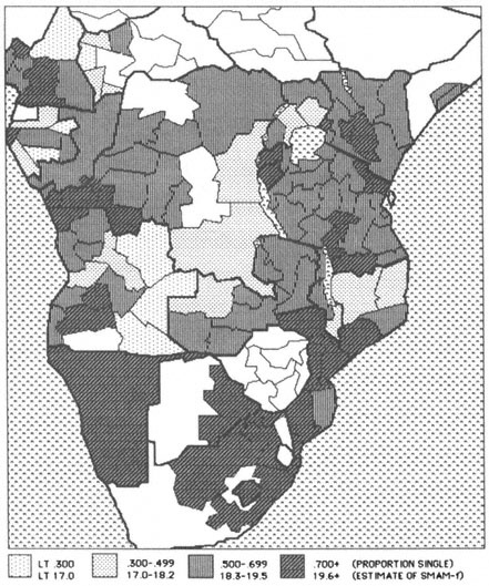
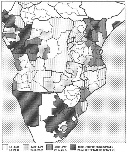
The first issues to be discussed are the ages at entry into a first union and the corresponding sex differential. The parameters used in map 6.2 are the proportions of single women 15–19 and the singulate mean age at marriage for women (SMAM-f ), which corresponds to this proportion according to the link established in eq. 6. 1. The following geographical pattern emerges:

1. A broad zone characterized by early marriage for women (SMAM values commonly below 18) lies in the western and central savannah and sahel regions, which contrast strikingly with a belt of later ages at marriage (commonly above 18 and often above 19.5) along the Atlantic. This Atlantic belt stretches all the way from Liberia to Namibia and is interrupted only in Gabon and Angola (provided that the data quality in these two countries was adequate in the 1960s). The inland boundary reaches from Monrovia in Liberia to Ilorin in Nigeria (Kwara state) and bends south to the Cameroon highlands, Congo, Bandundu province of Zaire, and Northwest Angola. The area of late female marriage continues with Southwest Angola until it reaches the Cape.

2. Several populations north of the sahelian strip of low female ages at marriage have higher values. This pertains particularly to Saharan nomadic groups who are often related to North African Berbers (for example, Hassania of Mauritania, Twareg).

3. There is a second strip of ages at marriage above age 18 for women covering much of East and South Africa. It contains pockets with SMAM values above 19 in Central Kenya, Rwanda, Burundi, and Northeast Tanzania. These pockets are welded together further south where ages at marriage above 19.5 become the rule in South African ethnic groups. Very recent survey data for the whole of Zimbabwe (1984) yield a SMAM value of just over 18, so that most of the blank area on map 6.2 for this country has presumably kept the Zambian pattern and has not yet adopted the South African system of very late marriage. Pockets of early marriage, that is, below 18, are also present in East Africa, for instance in Central Uganda, South Malawi, and North Mozambique.

4. It is not entirely clear whether the region of early female marriage in the western and central sahel still spreads along a north-south axis into Central Africa, as it did in the past. The data for Central, South, and East Zaire are old (that is, from 1955) and if a general trend toward later marriage has occurred, the contrast with West Zaire (data of 1975), Tanzania (1979), and Zambia (1969) may be artificial. Ages at marriage, however, in the Central African Republic, East Angola, and Northwest Zambia recorded in the 1960s further support the probable historical existence of such a central African area with SMAM values commonly lower than 18 years. If, on the other hand, mean ages at marriage have risen in central Africa, a general evolution towards a more simple dichotomy is probably underway, contrasting continued early marriage for women in the largely Islamized western and central savannah and sahel with mean ages at marriage over 18 for the rest of Africa.

Map 6.1a .
Statistical Areas, West Africa (see Key 6.1)

Map 6.1b .
Statistical Areas, East Africa (see Key 6.1)

5. Sudan, Ethiopia, and Somalia have been omitted from the discussion until now. Fragmentary evidence suggests than SMAM values for women were lower than 18 years in the 1960s, but recent surveys in Somalia and North Sudan (WFS) suggest a substantial rise. For North Sudan it is highly likely that this rise can, at least partially, be attributed to marital status–related age misstatement (cf. figure 6.1). Hence it is too early to come up with a definitive judgment regarding a recent trend.

The map with the male proportion single 20–24 or male SMAM values based on these proportions differs greatly from the map with the comparable female values (see maps 6.2 and 6.3). There is no western sahelian pattern of early marriage for men and the "Atlantic crescent" no longer provides a continuous string of late age at marriage (that is, above 25). The Central African north-south strip of early marriage for males (that is, below 25) extends well into East Africa, even if data from the late 1970s are used. The only major similarity with the distribution of female marital behavior is an overall pattern of late marriage for both sexes in South Africa, Botswana, and Namibia. The proportions single for the two sexes can be contrasted by means of the SMAM difference computed via equations 6.1 and 6.2. As indicated above, the lowest difference in husband-wife ages at first marriage is 3 years and the highest 11. Taking 7 years as a cutoff point, one can readily see on map 6.4 that the largest husband-wife differences are especially concentrated in West Africa. Differences in excess of 9 years (omitting Sudan, Ethiopia, and Somalia) only exist in the western Islamized areas, such as in Senegal, Guinea, and Central Burkina Faso. In East and South Africa, husband-wife age differences at first marriages between 7 and 9 years are only found in North Kenya and the Kenyan Rift Valley, and among the Tswana, Ndebele, and Venda ethnic groups of South Africa. Age differences in excess of 7 years are hence the rule in West Africa and the exception elsewhere. SMAM values computed on the basis of the full age schedule of proportions never-married or ratios of proportions single (RPS ) convey a similar picture.

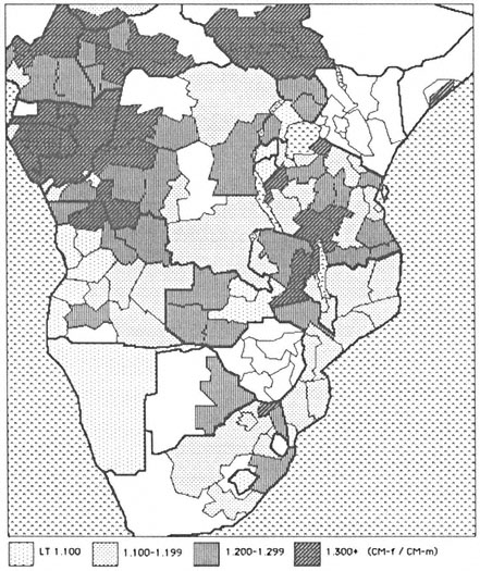
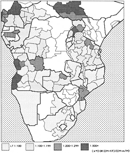
The geographic distribution of SMAM differences is obviously related to the pattern of polygyny. The comparison of map 6.4 showing the SMAM differences between the sexes with either map 6.5, showing the proportion of women currently married to a polygynist (f ), or map 6.6, with polygyny ratios (M ), testifies to this effect. The Atlantic polygyny zone stretches far inland and incorporates all climatic and cultural zones of West Africa. The high polygyny zone extends further south to Angola. The only Atlantic areas with less than 40 percent of married women in polygynous unions and polygyny ratios below 1.3 are found in Southeast Ivory Coast and Southwest Ghana (that is, in matrilineal Akan ethnic groups) and in the border regions of Southeast Nigeria and Southwest Cameroon. Finally, sahelian nomads

Map 6.2a .
Proportion Single Women Aged 15–19 and Approximate Values of the Female
Singulate Mean Age at First Marriage (SMAM-f); Latest Available Data

and Berber groups have a very low incidence of polygyny and do not fit the sub-Saharan pattern at all (see, for instance, Randall on the Tamasheq Twareg, 1984, and the WFS-results for the Hassania of Mauritania).

In general, the incidence of polygyny in Central, Eastern, and Southern Africa is much lower than in the Atlantic zone and the western sahel. There are, however, a few exceptions. Polygyny ratios above 1.20 or percentages of women married to polygynists in excess of 30 (still modest by West African standards) are found in West Kenya, Central Tanzania, East Zambia, North Malawi, and North Mozambique, forming an East African polygyny ridge that stretches south from Kisumu on Lake Victoria to the Tete province of Mozambique. In places along the coast of the Indian ocean values of M larger than 1.20 or f larger than 30 percent are also found: for example, in the Kenyan Coast province; the Tanzanian districts of Tanga, Lindi, Mtwara, and Ruvuma; the Mozambique province of Manica-Sofala; and among the coastal Nguni (Zulu) of South Africa.

The polygyny multiplier KL (that is, the ratio of proportions currently married of both sexes) and its major component L (that is, the ratio of proportions ever-married women and men) change the information given by the polygyny ratio M and the proportion of women in polygynous unions f to a considerable extent. One may recall from the previous section that KL is not positively affected by the adult sex ratio F/M. Consequently, areas with high values of M and f, but also with a substantial surplus of adult women, no

Map 6.2b .
Proportion Single Women Aged 15–19 and Approximate Values of the Female
Singulate Mean Age at First Marriage (SMAM-f); Latest Available Data

Map 6.3a .
Proportion Single Men Aged 20–24 and Approximate Values of the Male
Singulate Mean Age at First Marriage (SMAM-m); Latest Available Data

longer show up with dark shadings in map 6.7 presenting the polygyny multipliers. This results in the total disappearance of the East African polygyny ridge. With very few exceptions, polygyny multipliers do not exceed 1.20 in Central, East, and South Africa.

The picture for West African polygyny, measured by M or f, undergoes similar modifications if the polygyny multiplier KL is used. It should be noted, in passing, that KL values larger than 1.20 are the rule in West Africa, which makes the East-West contrast even sharper in map 6.7 than in the preceding polygyny maps. The map with polygyny multipliers closely resembles the map with SMAM differences (map 6.4). This is reflected in correlation coefficients: M and the sex difference in SMAM have a coefficient of 0.42, whereas KL and the SMAM -difference have a coefficient of 0.60.

Several of the West African areas that had been singled out for their relatively low incidence of polygyny (that is, Akan groups, Nigerian-Cameroon border area), no longer stand out once the polygyny multiplier is used. The KL values act to smooth out the data and present a more even picture.

Map 6.7 contains, however, one major exception: several regions in southern Nigeria with high values of M and f, have low values of KL. It is suspected that this exception is artificial: Nigerian sex ratios were obtained in the WFS household survey, whereas sex ratios for other countries are derived from censuses or much larger surveys. Given the small samples by state in the Nigerian WFS and the focus of attention on the fertility-oriented indi-

Map 6.3b .
Proportion Single Men Aged 20–24 and Approximate Values of the Male
Singulate Mean Age at First Marriage (SMAM-m); Latest Available Data

Map 6.4a .
Husband–Wife Age Difference at First Marriage; Latest Available Data

vidual questionnaire, an accurate recording of men in the household or elsewhere was less likely. An idea of the size of the error can be obtained from comparing the adult sex ratios in Cameroon as measured through the Cameroon WFS of 1978 and the census of 1979. This comparison is illustrated in table 6.4. The areas are ranked by surplus of women, from high to low, and the ratio between the two series indicates the relative magnitude of the deviation. These Cameroon data indicate that the ranking is similar for both sources, but that deviations by area can be as high as 16 percent. The largest

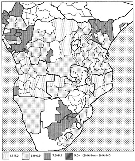
Map 6.4b .
Husband–Wife Age Difference at First Marriage: Latest Available Data

Map 6.5a .
Proportion of Currently Married Women Aged 15+ in Polygynous Unions

discrepancies are found in areas experiencing either considerable emigration (Western Highlands) or immigration (Southwest, Littoral). The WFS systematically produces a higher surplus of women, which is not surprising given that the main purpose of the household questionnaire was the identification of women of childbearing age. In Cameroon, greater care was taken to collect more detailed household-level information than in the other countries participating in the WFS, and it can be assumed that the WFS adult sex ratios for Cameroon are better than elsewhere. Morah (1985) compared the age specific sex ratios in the Nigerian WFS household data with those of the 1963 census and found a much larger excess of females in the age range from 15 to 60 in the national WFS-data set. In the age group 20–24, there were for instance 155 women per 100 men and in the age group 25–29 152 women. This anomalous pattern was less marked in the 1963 census with 119 and 114 women respectively. In view of this, it is entirely plausible to assume that the low KL values for southern Nigeria are the result of highly inflated sex ratios. Ogun state, for instance, has an adult sex-ratio for the entire population over 15 of 160 women per 100 men. The general conclusion is therefore that WFS data can be used to estimate values of f , but not for measuring M , KL , and sex ratios.

The issue of sex-ratio imbalances warrants further attention. There are two major sources of such imbalances: (1) measurement error as suspected, for instance, in the WFS household data, and (2) sex and marital status

Map 6.5b .
Proportion of Currently Married Women Aged 15+ in Polygynous Unions

Map 6.6a .
Polygyny Ratio; Latest Available Data

selective migration. Interaction between these two sources of variation may also occur. For instance, husbands who have migrated may accurately report the number of their wives but not specify their location. These women are then assumed to have migrated with them. If the wives are, however, in the area of origin, they risk being counted twice.

Most African migration streams are largely composed of men. The composition by marital status of the male migrants is more variable. The Voltaique migration to the Ivory Coast involves mainly single men, whereas the labor migration in South Africa involves all men. To what extent can the adult sex ratios of map 6.8 be explained in terms of migration? Table 6.5 contrasts the sex ratios of areas that are economically attractive with those of either neighboring zones of labor recruitment or economically disadvantaged areas. It is encouraging to find that the largest contrasts in adult sex ratios within countries are strongly associated with known migration streams and contrasts in regional population growth. Hence, the information in map 6.8 is not predominantly the product of measurement error.

The positive association between the polygyny ratio M and the adult sex ratio F/M (r = +0.50) has been given a specific interpretation in West African populations with a high incidence of polygyny. Capron and Kohler (1975) suggest that polygyny and male emigration are mutually reinforcing. This thesis is supported by data from the Mossi of Burkina Faso. The absence of young Mossi men gave the older, wealthier men, who remained at home, more opportunities for "monopolizing" the pool of available women.

Map 6.6b .
Polygyny Ratio; Latest Available Data

Map 6.7a .
Ratio of Proportions Currently Married 15+ or
Polygyny Multipliers; Latest Available Data

This resulted in bridewealth inflation and enhanced polygyny, consequently pushing more young Mossi to emigrate to the Ivory Coast in pursuit of means for financing the acquisition of a first wife. Strong gerontocratic control, polygyny with early marriage for girls, emigration of single men, and subsequent male marriage postponement formed the basic ingredients of this particular nuptiality regime. It is possible to imagine the alternative, the young migrants earning enough independently to compete with the older men in the marriage market. However, independent earnings are so strongly connected with a period of exile that even if the earnings are large enough, time abroad is still being lost, thereby resulting in a longer period of marriage postponement.

It would be dangerous to interpret the positive association between the polygyny ratio (M ) and the adult sex ratio exclusively in these terms. Alternatively, a surplus of married women is likely to be found wherever there is a surplus of women resulting from emigration of married males. Then, M is simply statistically contaminated by the adult sex ratio even in areas with much less polygyny.

The information presented in the various maps was compared and systematized through classic statistical procedures. First of all, it was considered fruitful to reduce the nine original indicators into a smaller number. This was done with a minimal loss of information by means of factor analysis. The underlying factors of the original set of indicators were defined in such a way

Map 6.7b .
Ratio of Proportions Currently Married 15+ or
Polygyny Multipliers; Latest Available Data

Map 6.8a .
Sex Ratios of Population Aged 15+ (Females/Males); Latest Available Data

that they bore no relation to each other (orthogonal factor extraction). In this instance, seven of the nine original indicators were used: the remaining two measure the differences in ages at marriage for men and women (SMAM difference and RPS ) and they are derived algebraically from the indicators of age at first marriage belonging to the first set. It was therefore statistically impossible to introduce them simultaneously with their components. Correlation coefficients of the SMAM difference and RPS with the factors defined by the first seven indicators were obtained subsequent to the factor extraction, and these values are reported in the bottom section of table 6.6.

The factor analysis results point to the existence of three major factors that jointly explain almost 80 percent of the original variance. Factor identification can be achieved through the single best indicators:

1. Factor 1 correlates strongly with the two measures of polygyny M and f . As expected, the correlations with the measures of the age gap at first marriage (SMAM difference and RPS ) are substantial. Those with the proportions single and with the adult sex ratio are equally logical in view of our previous discussion.

2. Factor 2 is identified by the adult sex ratio F/M. But, also a substantial negative association is found between L, that is, the main component of the polygyny multiplier, and factor 2. Moreover, this correlation is stronger than the one between L and the polygyny factor, which may seem surprising. At this point, it is necessary to recall that migration of

Map 6.8b .
Sex Ratios of Population Aged 15+ (Female/Males); Latest Available Data

TABLE 6.6  Major Underlying Dimensions of Sub-Saharan Nuptiality Indicators; Results from Factor Analysis   NOTE: Principle factoring (PA2) is used with VARIMAX and orthogonal rotation of factor axes.

single men distorts both the sex ratio and L in opposite directions: emigration of single men obviously raises the overall surplus of women and it increases the proportion of ever-married men, which is the denominator of L. Factor 2 can then be interpreted as carrying the effect of sex and marital status–differentiated migration. Equally noteworthy is the negative association between factor 2 and the SMAM difference (r = –0.52). If the effect of polygyny is factored out, a typical migration and marriage market feature emerges: for the overrepresented sex in an area, the proportion single below age 20 for women or 25 for men tends to increase and for the underrepresented sex it tends to decrease. In the instance of a female surplus, the corresponding SMAM values for women rise, whereas they fall for men. The correlation coefficients between factor 2 and the SMAM difference or RPS are entirely in line with this. It should, however, be stressed that proportions single and SMAM values are no longer valid indicators of ages at marriage in populations that are subject to substantial sex and marital status selective migration. Factor 2 correctly documents the concentration of young single

men in immigration areas, but one should be cautious in interpreting this as indicative of late marriage for men.

3. Factor 3 is identified by the two indicators of ages at first marriage. Both factor coefficients are positive: if polygyny and sex ratios are factored out, a geographical pattern remains that describes the overall timing of marriage for both sexes jointly.

4. The only indicator with low factor coefficients throughout is K. Evidently, the geography of the sex differences in proportions currently widowed and divorced constitutes a dimension on its own and accounts for a portion of the variance not explained by the three previous factors.

The ratio of proportions currently married K needs further discussion. It may be recalled that high values of K indicate a small surplus of the proportion widowed and divorced women in relation to the proportion widowed and divorced men. This is typically produced by a rapid relative pace of remarriage for women. K is furthermore less affected by sex-ratio distortions (r = –0.14), in contrast to L, the other component of the polygyny multiplier. Areas with a small relative surplus of proportions widows and divorcées are commonly found north of the line running from Douala in Cameroon to Cabo Delgado in Mozambique (K larger than 0.90), and areas with the smallest surplus (that is, K larger than 0.95) are almost exclusively found in West Africa. Such fast remarriage is consistent with high levels of polygyny in West Africa. On the other hand, large relative surpluses of widows and divorcées, that is, low values of K , are common in Zambia, Namibia, Lesotho, South Mozambique, and Botswana. This is equally consistent with low levels of polygyny and the presence of female-headed households instead. Mauritania has also low levels of K, fitting the low level of polygyny among its Arab population.

But there has been an enigmatic finding in the dominance of low levels of K in the area made up by South Cameroon, Gabon, Congo, and West Zaire, which is neither characterized by the existence of female-headed households, nor by low polygyny. In fact, it is the existence of this zone which prevents K from falling into a closer relationship with the other indicators of nuptiality and polygyny; further, this zone is responsible for the low factor coefficients of K reported in table 6.6.

Factor analysis has enabled the basic dimensions underlying the various nuptiality and polygyny indicators to be teased out. A few determinants were also collected for the regions and their effects were examined by multiple regression. The most important covariate is female literacy. Where actual measurement of illiteracy was missing it was measured as the proportion of women without formal schooling, in both cases for women 15–19. The information was limited to the youngest age group, primarily because most

first marriages for women occur before age 20. The proportion of illiterate women 15–19 also reflects the general level of illiteracy in the population and serves to distinguish those populations that have undergone a boost in female schooling and those which have not. The other covariates are the logarithm of population density and year of observation. Population density indicates the presence of urban concentrations, normally associated with higher ages at marriage for women and less polygyny. It also captures the presence of population concentration in rural areas which, often for geographic and climatic reasons, have had high population densities in the past (for example, Rwanda, Burundu, Central Kenyan Highlands, areas around Lake Victoria, and so forth). Population pressure in these rural areas is often considerable, and it is conjectured that this could result in the postponement of marriage. The year of observation is added to examine the effect of variation in the periods of observation.

The first set of dependent variables is made up of the indices of age at first marriage and the sex differences in these ages. The regression results are shown in table 6.7 in the form of beta-coefficients (that is, standardized regression coefficients). The zero-order correlations are provided for comparison. The results for the proportion of women single 15–19 and the ratio of proportions single (RPS ) are of necessity similar, given that RPS is influenced more by the proportion of women single 15–19 than the SMAM difference. The strongest determinant was female illiteracy, which exhibited the classic inverse relationship with proportions single women 15–19 and RPS: areas with high female illiteracy have earlier marriage for girls than areas with better schooling. This not only supports butjustifies the extension of the findings made in chapters 2 and 3 to the rest of sub-Saharan Africa.

The results for the variable "year of observation" were also significant: areas contributing recent observations tend to have later female marriage and higher RPS -values. But this should not be used as evidence of a rising trend in female age at marriage. Areas that are more developed socioeconomically also tend to have more recent data sources, while other, less developed areas are often described by a single, older source (such as Central African Republic, Chad, Bukina Faso, Mali, Guinea, South Sudan, East and North Zaire).

Male age at marriage and the SMAM difference were less affected by female literacy, but more so by polygyny. This reflects the fact that high male ages at marriage and the concomitant large age gap between spouses are almost exclusive to the West African polygyny belt. The extension of the study area beyond West Africa alters a finding of chapter 2, where a closer relationship between polygyny and female age at marriage was found. Hence, there is a plurality of factors associated with low ages at marriage for women and a more dominant single factor, that is, polygyny, associated with late marriage for men.

TABLE 6.7  Effects of Selected Variables on Measures of Age at First Marriage and Age Difference at First Marriage Dependent Variable   Zero-Order Correlations and Beta-Coefficients     Proportion Women 15–19 Illiterate Sex Ratio F/M Proportion Married Women in Polygynous Union Log of Population Density Year of Observation R2 R Proportion women 15–19 single               zero-order –.62 +.05 –.31 +.20 +.41     = .57  s= .20  beta –.63* +.03 +.06 –.07 +.39* .52 .72 Proportion men 20–24 single                 zero-order –.08 –.12 +.28 +.32 +.27     =.69 s =.13  beta –.42* –.28* +.60* +.21 +.01 .30 .54 Age difference at first Mariage                 zero-order +.40 –.21 +.53 +.19 –.01     =6.5 s = 1.6  beta +.04 –.36* +.59* +.04 –.06 .42 .65 Ratio proportion single women 15–19  to proportion single men 20–24 (RPS)                 zero-order –.62 +.17 –.49 –.01 +.27     = .83 s = .27 beta –.44* +.23* –.27* –.11 +.30* .53 .73 *Denotes significance at .05 level; N varies from 104 to 201.

Imbalances in adult sex ratios also have an impact on the proportion of single men 20–24 and the SMAM difference. A large surplus of women tends to lower male ages at marriage and the age difference between the spouses (cf. factor analysis results above). Population density, however, fails to produce significant results: the small positive zero-order correlations with both proportions single were as expected, but they vanish once literacy and polygyny are introduced.

The second set of dependent variables includes polygyny measures and the components of the polygyny multiplier. The regression results are shown in table 6.8. Attention is again directed to the effect of female schooling in view of the Westernization thesis of Goode and Caldwell. Despite the introduction of the proportion of women single 15–19, which is itself influenced by literacy, a strong positive and direct effect of female illiteracy on the polygyny indicators M and f is found. Areas with more literacy tend to have less polygyny, not only because women marry later in such areas, but also because of the direct polygyny-reducing effect of higher literacy. This is in line with Goode's hypothesis, but also consistent with Boserup's thesis that polygyny is a form of appropriation of female productive capacity in societies with traditional, low-technology agriculture. Given a negative relationship between subsistence agriculture and female education, one can indeed expect a negative association between female literacy and polygyny. The relationship between female illiteracy and the polygyny multiplier is smaller, but still in the direction suggested by Goode.

It is interesting to note the finding that higher female illiteracy is associated with higher K values, or with a smaller relative excess of widows and divorcées and faster remarriage of women. In other words, low literacy is associated with the minimization of the loss of reproductive capacity through celibacy, divorce, and widowhood.

The coefficients of proportions single are all in the expected direction and do not warrant further attention. Neither do the coefficients of the sex ratio since they show once more that the two types of polygyny measures (M and f versus KL and L ) are distorted in opposite directions. The coefficients of "year of observation" are nonsignificant throughout, and the effects of density on f and K essentially measure the East-West contrast.

The regional information for the components of the sub-Saharan nuptiality regimes can be summarized by the following:

1. With the exception of Arabs and Berbers, West African populations have considerably higher levels of polygyny, larger age gaps between spouses and faster remarriage then Central, East, and especially South African ones.

2. Islamized populations in West Africa have particularly early ages at marriage for women. This is partially due to high levels of female illiteracy. Non-Islamized populations of the region often reach similar

TABLE 6.8  Effects of Selected Variables on Measures of Polygyny and Components of the Polygyny Multiplier Dependent Variable Zero-Order Correlations and Beta-Coefficients   Proportion Women Single, 15–19 Proportion Men Single, 20–24 Proportion Women Illiterate, 15–19 Sex Ratio F/M Log of Population Density Year of Observation R2 R Proportion of married women in polygynous unions (f)   zero-order –.31 +.28 +.57 +.27 +.18 –.02     =.40   s = .14 beta –.20 +.42* +.54* +.40* +.28* –.09 .65 .80 Polygyny ratio (M)                   zero-order –.33 +.14 +.49 +.50 –.05 –.10     =1.28 s = .17 beta –.31* +.36* +.59* +.37* +.07 –.01 .63 .79 Polygyny multiplier (KL)                   zero-order –.34 +.32 +.52 –.54 +.13 +.05     =1.16 s =.16 beta –.30* +.30* +.36* –.44* +.05 +.01 .60 .77 Ratio of proportion ever-married (L)                   zero-order –.23 +.36 +.38 –.52 +.04 +.05     = 1.29 s = .15 beta –.35* +.50* +.16 –.45* –.15 +.09 .56 .75 Ratio of proportion currently married (K )                   zero-order –.25 +.01 +.39 –.14 +.24 +.01     =1.90 s =.07 beta +.02 –.06 +.44* –.07 +.36* –.10 .26 .51 * Denotes significance at .05 level; N varies from 104 to 201.

polygyny levels, but these are based on higher ages at marriage for women.

3. First marriage for men tends to be early in East Africa, which is in line with the more modest levels of polygyny. But male ages at marriage are particularly high in southern Africa, despite low polygyny levels. This undoubtedly reflects the disruption of traditional nuptiality patterns by vast male labor migration and the concomitant social and economic constraints on household formation typical for this region (see also chapter 8).

4. Male emigration is associated with enhanced polygyny in West Africa, but not in Southern Africa, where the response to it has been the emergence of female-headed households.

5. Apart from polygyny, the regional distribution of proportions single is also affected by migration and sex ratio distortions, largely because of the sex and marital status specificity of migration streams. Male emigration and the resultant surplus of women usually lead to enhanced proportions single among women 15–19 in the sending area. Conversely, in the receiving areas, males form the overrepresented sex with large accumulations of single males aged 20–34. SMAM values for regions experiencing heavy migration, in or out, do not reflect the real ages at first marriage of their individuals because of the violation of the stationarity hypothesis underlying the calculation of SMAM.

6. The cross-sectional associations of female literacy with female ages at marriage and polygyny are impressive and in the direction expected by Goode's thesis. They are, however, not directly interpretable as supporting Goode's proposition, which postulates, first, a causal link, and second, a general trend towards later marriage and less polygyny. There are "common causes" at work in the cross-section used so far, and these simultaneously affect female literacy, female age at marriage, and polygyny. For instance, simple technology in agriculture (that it, hoe agriculture) with heavy involvement of women is also correlated with low female literacy, early marriage, and high levels of polygyny (cf. Boserup's thesis). Islamization too depresses female literacy and enhances early female marriage as a result of the tighter control over women and partner selection (cf. Goody's thesis). The causal interpretation of the cross-sectional correlations between female literacy and the components of the nuptiality regime is, therefore, partially spurious since other social organizational variables are involved. Without statistical controls for these variables, the cross-sectional results are of limited use in inferring trends towards later marriage and less polygyny. What happens if such statistical controls are provided and if the traditional patterns of social organization are allowed to play their role? Before answering this question, a reformatting of the data according to ethnicity is required. This is taken up in the next section.

The Construction of an Ethnic Nuptiality and Social Structure File

As illustrated in chapter 2, patterns of social organization can be documented on the basis of ethnographic descriptions, and here further use is made of Murdock's Ethnographic Atlas. It was necessary to merge the demographic file, which was mostly region specific, and the ethnographic file, which was ethnic specific. The following principles were used to achieve such a merger:

1. Murdock classified each ethnic group in an ethnic cluster, thereby regrouping populations with similar linguistic, cultural, and organizational patterns. These clusters form the basic unit for establishing the correspondence between the two files.

2. Correspondence was first sought between individual ethnic groups and the regions for which demographic information was available. The matching was performed on the basis of ethnographic maps and the geographical coordinates given in the Ethnographic Atlas. This procedure works well in regions with a single dominant ethnic group. The matter is more complex, however, when a region holds a plurality of ethnic groups, or when an ethnic group is spread over several regions. To alleviate this problem, a nested design with differential weights was introduced.

3. The principles of this design were as follows. If an ethnic cluster was made up of, for example, four ethnic groups residing in areas with demographic information, each ethnic group was given a weight of 0.250. Within a cluster, weights always sum up to unity. If an ethnic group was spread over two regions with demographic information, its social structural characteristics were entered twice along with the two sets of demographic data for these two regions. The total weight for this ethnic group in the cluster was obviously maintained, but the two entries for the same ethnic group were given half this weight (for example, twice 0.125 instead of 0.250).

4. Two ethnic groups may reside in the same area. If they belonged to the same cultural cluster, as defined by Murdock, both received the same regional demographic information, either as their sole demographic input or as a partial input. In the latter instance, weights were further fragmented as outlined by principle 3. Regions with heterogeneity in terms of cluster membership were avoided as much as possible. This principle assured that the correspondence between regions and ethnic clusters was maximized in instances where correspondence between regions and ethnic groups was imperfect.

5. A few deviations were tolerated. The Fulani, Twareg and northern (or "nuclear") Mande groups are spread over much of the West African sahel and savannah, and the ethnic entries in the Murdock file for these

Map 6.9a .
Correspondence Between Areas with Demographic Information and Location of Ethnic Clusters

groups pertain to three particular populations that fall outside the regions with demographic information. In these instances, the ethnographic information was maintained and coupled with demographic information from the Fulani, Twareg, and northern Mande groups elsewhere. A second alteration was performed on Murdock's "Coastal Nigeria" cluster, which was broken up into a new cluster (Bendel) and a set of ethnic groups which were attached to the existing "Cross River" cluster. This new configuration is ethnically more homogeneous and covered fully by demographic information.

6. In instances where demographic information was already ethnic specific (such as Burkina Faso, Gabon, South Africa, most WFS-participating countries) the above problems were absent and a direct match was made.

The outcome of the matching process is shown in map 6.9 for the clusters. The data file contains entries for 170 ethnic groups nested in 69 clusters. The ratio is 2.46 groups per cluster. In further statistical work, all weights were inflated by this ratio in order to respect the real sample size (N = 170) without distorting the nested design.

The following demographic variables were entered:

1. The proportions single women 15–19 and men 20–24. The approximate SMAM values were computed through the conversion formulae given earlier and an estimate of the sex difference in SMAM was added.

Map 6.9b.
 Correspondence Between Areas with Demographic Information and Location of Ethnic Clusters

2. Polygyny is measured through the same indices as before, but for the cases without entries for the proportion of married women in polygynous unions ( f ), values were estimated on the basis of the polygyny ratio (M ) in accordance with the regression of f on M (r = 0.75; N = 119 entries). Obviously, this estimation was performed to reduce the number of missing values, which would otherwise lead to a serious selection bias. Hence, the selection bias associated with missing values was considered to be more hazardous than the approximation of f through M.

3. Additional demographic variables are the adult sex ratio (F/M ) and population density. Also the period of observation was added.

The file contains the following ethnographic data:

1. The Murdock scales of the degree of subsistence dependence on respectively hunting/gathering, fishing, animal husbandry, and farming. These scales can be interpreted as the degree (expressed in percentages) of subsistence reliance on any of these sectors.

2. The pattern of exchange of goods and services on the occasion of marriage (EXCH MAR) was measured through the entries in column 12 of the Murdock file and recoded as follows:

0: no exchange or token exchange only (O,T)

1: prestations from the groom's lineage to the bride's lineage (i.e., bridewealth, bride-service, and sister exchange; B,S,X)

2: reciprocal exchange of substantial gifts (G)

3: transfers from the bride's lineage to the new household or the groom's lineage (i.e., dowry; D)

3. The pattern of residence of wives (MARRES) is based on Murdock's column 16 and recorded as:

0: no common residence (O)

1: uxorilocal or matrilocal (U,C,M,A)

2: neolocal (N)

3: virilocal or patrilocal (P,V,D)

4. Lineage organization (LIN) stems from columns 20, 22, and 25 (second digit):

1: strong patrilineal (0 in 22, not in 20, a in 25)

2: patrilineal (0 in 22, not in 20, not a in 25)

3: matrilineal (0 in 20, not in 22, not m in 25)

4: strong matrilineal (0 in 20, not in 22, m in 25)

5: duo + bilateral (0 in 20 and 22 or not 0 in 20 and 22)

In further statistical work codes 1 and 2 are merged to identify patrilinearity and 3 and 4 are regrouped to indicate matrilinearity.

5. The tolerance of or preference for cousin marriages (COUSMAR) are taken from column 25 and coded as follows:

1: no cousin marriage of any kind (N,O,R,S)

2: patrilateral cousin marriage (P,D)

3: evidence of matrilateral cousin marriage (M,G)

4: duolateral, trilateral, and quadrilateral cousin marriage (C,T,Q).

Endogamous marriage is identified by combining the variables "Lineage organization" and "cousin marriage." All societies without cousin marriage of any sort are obviously exogamous. Those with patrilineal organization and patrilateral cousin marriage, matrilineal organization and matrilateral cousin marriage, and those with multilateral cousin marriage are considered as tolerating endogamy (it must be noted, however, that trilateral cousin marriage is an exception and is exogamous).

6. The degree of political complexity (POLCOMP) is obtained from column 32 (second digit):

0: stateless societies

1: existence of petty chiefs

2: existence of large paramount chiefs

3: states

4: large states

Note that Murdock has excluded patterns of political organization introduced by colonial authorities.

7. The variable describing "community size" was directly taken from the Murdock files (column 31), with codes ranging from 1 to 8. The distinctions between the lower codes (1 to 6) do not appear to be very meaningful and the scale can be dichotomized on the basis of the existence of indigenous cities (code 1–6 versus 7,8).

8. Murdock provides a code for the female involvement in agricultural work (FWAGRIC) (column 62). These were recoded as:

0: agriculture of no importance

1: males do more agricultural work than women (M,N)

2: both sexes are equally involved (E,D)

3: females do more agricultural work (F,G)

This variable is important in testing Boserup's proposition (see later discussion), but, as argued by Goody (1976), the validity of this variable is reduced when the analysis is confined to sub-Saharan populations only. In many such societies with entries specifying less female agricultural involvement or equal division of labor, women are involved in trading as well, which enhances their "productive value."

9. The existence of caste and/or class stratification (CCS) is taken from Murdock's columns 67 and 69:

1: unstratified by caste or class (0 in 67 and 69)

2: stratification by wealth only (W in 67, 0 in 69)

3: some despised social groups (0 in 67, D in 69 or D in 67, 0 in 69)

4: moderately stratified (E in 67 or D,E in 69)

5: heavily stratified (C in 67 or 69)

For sub-Saharan populations, a dichotomy can be formed by adding the societies with despised groups, of which there are normally only one or two, to the category of unstratified societies. The numerical share of such groups is very small and the label "despised" is not always accurate since some groups (for example, blacksmiths) are often endowed with magic powers. Obviously, stratification by age grades or other forms of gerontocratic rule are not considered as forms of class or caste stratification.

10. The possibility of women inheriting property is given in Murdock's columns 74 for real property (REAL) and column 76 for movable property other than kitchen utensils and the like (MOVE). The codes are:

1: women inherit (C,D)

2: women do not inherit (M,N,O,P,Q)

Major Anthropological Theories and Their Empirical Testing

At this juncture, it is necessary to review the anthropological theories that form the basis for the interpretation of the collected data. In figure 6.13, use is made of six explanatory variables measuring respectively the degree of subsistence dependence on agriculture and female labor inputs, the format of lineage organization, the presence of forms of diverging devolution of property through women, the degree of political complexity, the extent of social stratification, and female literacy. These factors are considered to influence male and female ages at marriage, either directly (paths A and C) or indirectly through the incidence of polygyny and its corollary, the age gap between spouses (paths B, D, G, and H).

Although anthropologists documented the existence and practice of polygyny in early research (see, for example, Radcliffe-Brown and Forde, 1950), little attempt was made to explain its occurrence. Inasmuch as structural functionalist anthropology drew elegant, holistic pictures of discrete societies, it tended not to engage in extensive comparative approaches. Only with the advent of the Murdock Ethnographic Atlas and demographic measurements did this become a real possibility.

It was an economist, Ester Boserup (1970), who first attempted a comparative overview of the relationship of social features such as nuptiality to organizational and economic variables. Boserup's thesis is straightforward:

Figure 6.13.
Variables Involved in Statistical Analyses of Ethnic Marriage Regimes

farming systems can be divided into male and female systems. In areas of low population density, such as sub-Saharan Africa, Boserup postulated that shifting cultivation using the hoe and female labor, would be practiced. Any other female economic contribution, such as trading in West Africa, would be added to the productive value of women. Women's high economic value would therefore be reflected in high levels of polygyny, fast remarriage for widows (appropriation of female labor in gerontocratically structured societies), and bridewealth. The alternative is a system where men do the agricultural work with more advanced technology (irrigation, plough) and the women's reduced contribution would be reflected in monogamy, less remarriage, and dowry. In sum, Boserup viewed marital practice as being a function of the relative contribution of the sexes in agricultural production, and the operationalization of her thesis would essentially occur via paths B and D in figure 6.13.

As shown in chapter 1, Goody (1976) put Boserup's thesis to the test and found that, in general, it held well when run against Murdock's ethnographic information. In fact, Goody's own thesis is similar and goes one step further. For Goody, the transmission of property becomes the deciding factor in the social and economic system. In low-technology hoe agriculture, land is corporately owned and widely available, and its transmission is not a grave issue since all lineage members have access to it. Marriage payments in such a

system, that is, bridewealth, are not so much concerned with the transmission of property, but with the transmission of the productive and reproductive value of women. In systems with more advanced plough agriculture, property, states, castes, and other forms of social stratification based on wealth are predicted. The system evolves away from the principle of circulation of resources towards concentration of wealth. In order to protect these interests, marriage tends to become endogamous. This is also an answer to the practice of bilateral inheritance. A father who wishes to protect his daughter's status with a dowry, but keep the family property intact, may solve the problem with caste or lineage endogamy. In-marriage implies strong parental control with respect to partner choice and avoidance of premarital conceptions or births. In many instances that are not characterized by neolocal residence, this leads to the marrying off of women at young ages. Goody's mechanism operates essentially via path A in figure 6.13.

Similarly, Goody's thesis divides the world essentially into two: those societies with diverging devolution of property through bilateral inheritance, dowry, monogamy, plough agriculture, complex polity, and social stratification, versus those with unilineal descent groups, bridewealth, polygyny, shifting cultivation with hoe technology, and high female labor inputs in agriculture. In this fashion, he also incorporates Boserup's dichotomy.

The testing of Goody's and Boserup's thesis with a sub-Saharan rather than a worldwide sample faces the problem of increased homogeneity with respect to the social organization variables. Bridewealth, for instance, constitutes by far the most common form of marriage prestation (86 percent of entries in our data file), irrespective of the form of lineage organization. The practice of dowry is virtually absent, and the remaining 14 percent of societies without bridewealth are distributed over the categories of no exchange, token exchange only, gift exchange, bride-service, or sister exchange. Inheritance for women is rare and occurs in 20 percent of the entries. Tolerance of or preference for endogamous forms of cousin marriage is more common (mostly of the bilateral, trilateral, or quadrilateral types) with 46 percent of entries, but the combination with inheritance for women results in few societies that manifestly counteract diverging devolution of property through endogamy. In fact, this combination is found in twenty-nine societies only, or seventeen percent of the entries. Hence, the few that have inheritance for women generally tolerate endogamous marriage, but those who tolerate cousin marriage do not necessarily practice inheritance for women. Of the twenty-nine societies with both diverging devolution of property and endogamy, twenty-one are thoroughly Islamized, which presumably explains the origin of this non-African combination. None of the remaining eight societies are patrilineal and hence they are exceptional in more than one respect.

As Comaroff (1980) pointed out, what is the use of the Boserup-Goody

generalized distinction, when so much of Africa falls in a single category? Hence, additional explanatory variables have to be found with more discriminating power for this continent. Goody (1973) himself, in an earlier critique of Boserup, stressed that female involvement in agricultural production itself would not suffice to explain marriage patterns. As Comaroff underlines, the problem with assigning "value" to women according to their productive potential begs the question of what kinds of female and male activities are regarded as valuable. There may be a crucial distinction between the actual economic contribution of the sexes with respect to the production of means of subsistence and the socially perceived contribution. For example, in many African societies, which rely predominantly on agriculture, animal husbandry is also practiced, and in these the socially perceived value of female agricultural work is often lower relative to the inflated value ascribed to the male involvement in cattle raising and trading. This relationship is typical to East Africa, where cattle raising is common and women seldom engage in trading activities.

The relevant distribution characteristics in the data file are as follows: the modal category for reliance on agriculture is comprised of between 50 and 69 percent dependence on this sector and contains 61 percent of the entries. Of these, half the number of entries have scores indicative of greater female than male labor involvement in agriculture. The modal category for animal husbandry is 6–25 percent reliance with 55 percent of entries. Hence, the combination of a dominant farming sector with an additional cattle raising one is not rare and the same probably holds true for the social devaluation of women's economic contribution.

To sum up, the Murdock variables relating to the degree of subsistence reliance by sector and to the female work input in agriculture do not constitute an optimal measurement of the dimension of the perceived value of women. This is most clearly visible in the fact that the variable of female versus male farming does not discriminate between East and West Africa, whereas the social value of women's work and the social position of women are known to be weaker in East Africa. The reliance on animal husbandry versus agriculture may be a better proxy than the direct female work input in agriculture used by Boserup, because of the prestige associated with cattle owning accruing to men only. The hypothesis to be tested is then that increased reliance on farming and decreased importance of animal husbandry leads to greater perceived productive value of women and to more polygyny and larger age gaps between the spouses (paths B, D in figure 6.13).

Another essential element that should be included in the explanatory framework is the relationship between lineage organization and polygyny. One might predict that matrilineal societies would be less polygynous because of problems with household formation. Matrilineal societies that have matrilocal or uxorilocal residence of spouses impede polygyny since the hus-

band would have to marry sisters. In the present data file, 18 percent of societies are matrilineal, of which two thirds have matri- or uxorilocal residence. As a consequence, one can indeed expect that societies with matrilineal descent systems would be less polygynous, have smaller age gaps between the spouses, and have either later marriage for women and/or earlier marriage for men (effect through paths B, D, G, and H in figure 6.13).

The effects shown in figure 6.13 were statistically tested and measured as follows. Two sets of tables were prepared, respectively excluding and including polygyny as a predictor. In the first set the direct effects A, B, and C in figure 6.13 proved of interest, whereas the results of the second set also take the existence of D, G, and H into account. Each set is composed of three tables. The first table in each set (that is, tables 6.9 and 6.12) gives the results of an analysis of variance and permits a comparison of the proportions of variance of each of the four dependent variables (proportions single women 15–19, proportions single men 20–24, SMAM difference inferred from these proportions, proportion married women 15+ in polygynous unions) accounted for by the independent variables listed in figure 6.13. The year of observation has been added to the set of predictors merely as a control for differential data quality over time. The five social organization variables are discrete (factors), whereas female literacy and the year of observation are continuous (covariates). In the second set of tables, the incidence of polygyny is added as a covariate. The second table in each set (that is, tables 6.10 and 6.13) contains the results of a Multiple Classification Analysis (MCA) corresponding with the analyses of variance. In all these analyses missing values have been deleted in a listwise fashion, which means that a missing value for any of the variables results in the deletion of the case from the file. Listwise deletion produces a substantial loss of cases and sample sizes are reduced from 170 to 107–121 depending on the dependent variable. The third table in each set (that is, tables 6.11 and 6.14) shows the unstandardized regression coefficients from a dummy regression analysis. As no interaction terms are considered, the column with "adjusted deviations" in the MCA tables and the regression coefficients should reveal, each in its own way, a similar picture. However, the dummy regression procedure used here is based on pairwise deletion of missing values, meaning that a case is only omitted from a bivariate relationship as a result of a missing value. The procedure minimizes the loss of cases, but bivariate relations are rarely computed on the basis of identical samples. These two different treatments of missing values serve to check whether results display sufficient robustness against the selection bias produced by missing data. Finally, one should be reminded of the fact that the nested design and its weighting procedure are used throughout these analyses (see earlier discussion).

The first set of tables which exclude polygyny as a predictor are now considered (tables 6.9 through 6. 11). The independent variables provide the

TABLE 6.10 Effects of Social Organization Indicators on Four Nuptiality Variables: Results of Multiple Classification Analyses Excluding Polygyny as a Covariate for Age-at-First-Marriage Variables; Sub-Saharan Ethnic Clusters   Proportion Women single, 15–19 Proportion Men Single, 20–24 SMAM Difference Proportion Married Women in Polygynous Unions   = .57 = .70 = 6.61 = .37   N = 118 N = 108 N = 108 N = 121   Unadjusted deviation Adjusted deviation N Unadjusted deviation Adjusted deviation N Unadjusted deviation Adjusted deviation N Unadjusted deviation Adjusted deviation N Factors                                                   Pastoralism/Agriculture                       Pastoral –.07   .06 (8) –.07 –.03 (6) –.67 –1.50 (6) –.10 –.14 (9) Mixed (pastoral, hunter-gatherer, agriculture –.01 –.04 (28)   .02   .01 (25)   .43     .54 (25) –.03 –.03 (28) Medium   .01   .01 (74) –.00   .00 (70) –.08   –.06 (70)   .01   .02 (76) agriculture                         High agriculture   .04 –.03 (7)   .01   .02 (7) –.16   –.04 (7)   .07   .04 (8) eta/beta        .10        .14          .13        .08          .17        .27          .25        .33   Lineage Organization                         Patrilineal –.01 –.00 (79)   .00   .01 (71)   .10     .09 (71)   .02   .03 (81) Matrilineal   .02   .02 (23) –.03 –.02 (23) –.48   –.31 (23) –.09 –.10 (23) Bilateral and    duolateal –.00 –.02 (16)   .02   .00 (14)   .29     .07 (14)   .02   .01 (16)       eta/beta        .05       .06         .11       .08         .16        .10            .30         .35

Proportion Women single, 15–19 Proportion Men Single, 20–24 SMAM Difference Proportion Married Women in Polygynous Unions   = .57 = .70 = 6.61 = .37   N = 118 N = 108 N = 108 N = 121   Unadjusted deviation Adjusted deviation N Unadjusted deviation Adjusted deviation N Unadjusted deviation Adjusted deviation N Unadjusted deviation Adjusted deviation N Diverging Devolution of Property                     No inheritance by women   .02   .01 (102)   .00   .00 (91) –.13 –.08 (91)   .00   .00 (105) Diverging devolution through women + endogamy –.12 –.07 (16) –.00 –.01 (16)   .76   .43 (16) –.02 –.02 (15) eta/beta       .23          .14         .01       .03         .20       .11         .04       .05   Political Complexity                         No chiefs or minor local chiefs –.03 –.04 (68) –.01 –.01 (61)   .05   .11 (61)   .01   .02 (70) Paramount chiefs and states   .05   .05 (50)   .01   .01 (47) –.06 –.14 (47) –.02 –.02 (50) eta/beta       .19       .20         .09       .06         .03       .08         .12       .15   Class and Caste Stratification                       Unstratified or despised group only   .02 –.00 (69) –.02 –.02 (63) –.36 –.20 (63) –.00   .00 (72) Stratified (wealth or castes) –.03   .01 (49)   .02   .03 (45)   .50   .28 (45)   .01 –.00 (49) eta/beta      .13       .03         .15        .20         .27       .15          .01        .02   NOTE: "Adjusted deviations" measure deviations from the overall mean adjusted for all other factors and 2 covariates (literacy women 15–19 and year of observation). See also note for table 6.9.

TABLE 6.11  Effect of Social Organization Variables and Female Literacy on Nuptiality and Polygyny in Sub-Saharan Ethnic Clusters; Unstandardized Regression Coefficients   Proportion Women Single, 15–19 Proportion Men Single, 20–24 SMAM Difference in Years Proportion Married Women in Polygynous Union   = .55 s = .22 = .69 s = .14 = 6.57 s = 1.52 = .36 s = .14                   Social Organization Variables                 Pastoralism/Agriculture                 Pastoral       Reference Group       Mixed (pastoral, hunter-gatherer, agriculture) –.08 +.00 +.82 +.14* Medium dependency agriculture –.06 –.00 +.56 +.20* High dependency agriculture –.07 –.01 +.45 +.21* Lineage Organization                 Patrilineal       Reference Group       Matrilineal +.01 –.02 –.37 – .11* Bilateral and duolateral +.00 –.06 –.11 –.03 Diverging Devolution of Property                 No diverging devolution & exogamy       Reference Group       Women inheritance, edogamy –.07 –.02 +.13 –.04* Political Complexity                 No chiefs or local chiefs only       Reference Group       Paramount chiefs or states +.06* +.09 –.23 –.05*

Proportion Women Single, 15–19 Proportion Men Single, 20–24 SMAM Difference in Years Proportion Married Women in Polygynous Union   = .55 s = .22 = .69 s = .14 = 6.57 s = 1.52 = .36 s = .14 Class and Caste stratification                 None or despised group only       Reference Group       Class or caste stratified +.02 +.07* +.13 –.00 Other Variables (Continuous) Female literacy (proportion)     +.441* +.078    –2.019*    –.132* Year of observation (55–82)   +.003 +.005*     +.042* +.002 Regression Constant     .557 .352   1.625    .021 R   .68 .43   .51 .56 R2   .47 .18   .26 .31 NOTE: In contrast to MCA-results, regression outcomes are based on pairwise rather than listwise deletion of missing variables so that Ns are comprised between 142 and 170 (maximum). Asterisks denote significance at .05 level.

best prediction in the instance of ethnic variation in proportions single women 15–19 (R² = 0.46). Much of this is attributable to the positive effect of female literacy, which accounts for 28 percent of the variance in proportions single. Ethnic variation in female ages at first marriage is consequently essentially related to the modernizing effect of higher female literacy in this cross-section. This is entirely in line with all the earlier findings (see chapters 2 and 3). The other significant, but much smaller, proportions of the explained variance stem from diverging devolution coupled with endogamy (6 percent) and political complexity (6 percent). Table 6.10 with the corresponding MCA results shows the magnitude and the direction of the effects. As expected, the few societies with both inheritance for women and tolerance and/or preference for endogamy have substantially lower proportions of single women 15–19. Not adjusting for the other variables, their mean proportion is 0.57 – 0.12 = 0.45 as opposed to 0.57 + 0.02 = 0.59 in societies without diverging devolution of property through bilateral inheritance. The original discrepancy of 14 percentage points is reduced to 8 percentage points if the other variables (including literacy) are controlled for, but the difference nevertheless remains significant. Since very much the same result is obtained in table 6.11, this finding does not stem from the specific treatment of missing values. Hence, Goody's variables of property transmission and control over young women identify the pattern of particularly early marriage for girls in societies that are mostly profoundly Islamized and perform exactly according to the theory. The effect of political complexity stems from later marriage in societies that have paramount chiefs or states. This is also in line with a similar (although nonsignificant) effect of enhanced stratification.

A quarter of the variance of polygyny is accounted for by the set of predictors used here. The effect of female literacy is much smaller (0.04) than in the instance of female age at first marriage (0.28), but the effects of subsistence dependence on cattle or agriculture and of lineage organization emerge more clearly (0.10), as would be expected from the theoretical propositions. The reduced effect of female literacy contrasts with the finding in chapter 2 where female schooling levels played a far more prominent role. Admittedly, literacy and schooling level are not identical variables, but the main source of the reduction in the explanatory power of literacy is the extension of the present sample to most of sub-Saharan Africa in contrast to the predominantly West-African sample used in chapters 2 and 3. However, as can be seen from the dummy regression results reported in table 6.11, polygyny and literacy are still negatively related. The magnitude of the coefficient (–0.132) indicates that a 10-percentage-point shift in female literacy produces on average a diminution of the percentage of married women in polygynous unions of 1.3 points. Considering that the respective means for polygyny and literacy are 36 and 45 percent, and the respective standard deviations are 14 and 30 percent, this cross-sectional slope indicates that polygyny would on average

TABLE 6.13 Effects of Social Organization Indicators on Three Nuptiality Variables: Results of Multiple Classification Analyses (Including Effect of Polygyny); Sub-Saharan Ethnic Clusters   Proportion Women Single, 15–19 Proportion Men Single, 20–24 SMAM Difference   = .57 =.70 = 6.60   N3 = 117 N3 = 107 N = 107   Unadjusted deviation Adjusted deviation N Unadjusted deviation Adjusted deviation N Unadjusted deviation Adjusted deviation N Factors                   Pastoralism/Agriculture                   Pastoral –.07    .03 (8) –.07 .01 (6) –.66 –.78 (6) Mixed (pastoral, hunter-gatherer, agriculture)    .00 –.04 (27)    .02 .03 (23)   .42   .66 (23) Medium agriculture    .00    .01 (74) –.00 –.01 (70) –.07 –.14 (70) High agriculture    .04 –.02 (7)    .01 –.03 (7) –.15 –.16 (7) eta/beta    .10    .11      .14   .11     .16   .24   Lineage Organization                   Patrilineal –.00    .00 (78)     .01    .00 (70)   .09   .00 (70) Matrilineal    .02    .00 (23) –.03    .00 (23) –.47 –.03 (23) Bilateral and duolateral –.01 –.02 (16)    .02 –.01 (14)   .30   .02 (14) eta/beta    .04   .05      .11   .03     .16   .01   Diverging Devolution of Property                   No inheritance by women   .02   .01 (102) –.00 –.00 (91) –.13 –.09 (91) Diverging devolution + endogamy –.11 –.06 (15)    .00    .01 (15)   .78   .56 (15) eta/beta    .20     .11        .01    .02      .20 .14

Proportion Women Single, 15–19 Proportion Men Single, 20–24 SMAM Difference   = .57 =.70 = 6.60   N3 = 117 N3 = 107 N = 107   Unadjusted deviation Adjusted deviation N Unadjusted deviation Adjusted deviation N Unadjusted deviation Adjusted deviation N Political Complexity                   No chiefs or minor local chiefs –.03 –.03 (66) –.01 –.01 (60) .04   .10 (60) Paramount chiefs and states   .04   .04 (50)   .01   .01 (47) –.05 –.12 (47) eta/beta   .18   .17     .08   .05     .03   .07   Class and Caste Stratification                   Unstratified or despised group only   .02 –.01 (69) –.02 –.03 (63) –.35 –.25 (63) Class or caste stratified –.03   .01 (48)   .03   .04 (43)   .51   .36 (43) eta/beta   .12   .04     .16   .24     .26   .19   NOTE: "Adjusted deviations" measure deviations from the overall mean adjusted for all other factors and covariates (literacy women 15–19, year of observation, and proportion of married women in polygynous unions). See also notes for table 6.9.

TABLE 6.14  Effect of Social Organization Variables, Female Literacy, and Polygyny on Age-at-First-Marriage Variables in Sub-Saharan Ethnic Clusters; Unstandardized Regression Coefficients   Proportion Women Single, 15–19 Proportion Men Single, 20–24 SMAM Difference   = .55 s = .22 = .69 s = .14 = 6.57 s = 1.52 Social Organization Variables             Pastoralism/Agriculture             Pastoral     Reference Group     Mixed (pastoral, hunter-gatherer, agriculture) –.04 –.02 +.34 Medium dependency agriculture –.01 –.03 –.13 High dependency agriculture –.01 –.05 –.29 Lineage Organization           Patrilineal     Reference Group     Matrilineal –.02 –.01 –.00 Bilateral and duolateral –.01 –.00 –.01 Diverging Devolution of Property             No diverging devolution & exogamy     Reference Group     Women inherit, endogamy –.08 –.02 +.26 Political Complexity             No chiefs or local chiefs only     Reference Group     Paramount chiefs or states +.05 +.02 –.04 Class and Caste Stratification             None or despised group only     Reference Group     Class or caste stratified +.02 +.07* +.71*

Proportion Women Single, 15–19 Proportion Men Single, 20–24 SMAM Difference   = .55 s = .22 = .69 s = .14 = 6.57 s = 1.52 Other Variables (Continuous)           Female Literacy (proportion) +.406* +.100* –1.557* Year of Observation (55–82) +.004 +.004*   +.035* Married Women in Polygynous Unions (proportions) –.262* +.167 +3.494* Regression Constant   .582   .349   1.552 R   .70   .45     .57 R2   .48   .20     .32 NOTE: In contrast to MCA-results, regression outcomes are based on pairwise rather than listwise deletion of missing variables so that Ns are comprised between 142 and 170 (maximum). Asterisks denote significance at .05 level.

still occur at the 31 percent level in societies with 80 percent female literacy and at the 29 percent level in instances of complete female literacy. Hence, the sign of the slope is in line with Goode's expectation, but its size points in the direction of the robustness of the institution, as hypothesized by van de Walle and Kekovole (1984). This discussion on the relationship between literacy and polygyny cannot be complete without the warning that cross-sectional results are no substitutes for trends over time, notwithstanding the controls for traditional social organization variables.

The effect of the variable measuring the importance of cattle raising versus agriculture produces, as indicated, a major effect: it accounts for 10 percent of the variance in polygyny, and the differences between the extreme categories (pastoral versus sole dependence on agriculture) amounts to an average of 18 percentage points more polygyny for the agricultural societies in the MCA analysis (table 6.10) and to 21 percentage points in the dummy regression analysis (table 6.11). Polygyny increases also monotonically with the growth of agriculture. This is clearly "within-Africa" evidence supportive of Boserup's thesis that increased activity in low-technology swidden agriculture enhances the productive value of women and fosters polygyny. The contrast with cattle raising societies, where women are perceived as "uneconomic" and polygyny is lower, accounts partially for the contrast in the incidence of polygyny between West and East Africa (cf. maps 6.5, 6.6, and 6.7).

The two organizational features that tend to reduce polygyny and which statistically curb the polygyny enhancing effect of greater involvement in low-technology agriculture are matrilineal kinship organization and aspects associated with the emergence of social stratification. The lineage factor explains 13 percent of the variance of polygyny (table 6.9), which is as much as agriculture (0.10) and much more than female literacy (0.004). The entire effect of lineage is due to the category of matrilinearity as shown by the MCA and dummy regression results (tables 6.10 and 6. 11). The order of magnitude of the effect is equally important: matrilinearity produces on average a 13-percentage-point diminution in polygyny when compared to patrilineal descent systems. This is confirmed by the dummy variable regression with a shift of 11 percentage points. This corresponds almost to a full standard deviation shift toward the lower end of the polygyny distribution. The finding is in accordance with the theoretical proposition that matrilineal systems would have an additional problem with polygynous household formation as a result of their tendency toward matrilocal or uxorilocal residence. The result also suggests that matrilineal descent should be added to the Boserup-Goody list of explanatory variables, especially when dealing with low-technology farming societies.

The three variables that are connected with the emergence of social stratification in function of wealth or descent (that is, diverging devolution and endogamy, political complexity, and class or caste stratification) also have a

negative effect on polygyny, but the magnitudes are smaller. The finding is again in line with Goody's view that monogamy becomes the rule in more complex societies with bilateral transmission of property and a concern for endogamy and homogamy. There are several reasons accounting for this negative relationship:

1. A simple gerontocratic structure is most propitious for polygyny as this practice involves the appropriation of female productive and reproductive functions by older men. Deviations from such gerontocratic organization generally imply complications for the maintenance of high levels of polygyny.

2. A stratification system based on wealth and descent leads to the fragmentation of the marriage market and imposes problems in the recruitment of suitable brides.

3. If hypergamy is desirable, plural marriages increase the chances of hypogamy. If the top stratum is highly polygynous, more single men of this stratum may be inclined to take a bride from the next lower stratum rather than remain single for a longer time. This in turn creates a deficiency of available brides in the second stratum and in the presence of polygyny, more men of the second stratum may again have to resort to hypogamy. Each man who succeeds in recruiting a bride from a higher class or caste is effectively imposing a match with a woman of a lower stratum on someone else. This externality arising from a deviation from perfect homogamy is contained by monogamy and exacerbated by polygyny.

There are, however, several societies in the sample which have a dual caste system combined with high levels of polygyny. One of these, the sedentary Fulani or Peul, has been thoroughly studied by G. Pison (1982, 1986). Typical of Goody's "Asian" pattern is that the Fulani (Pison studies the Bandé subgroup located in Senegal) have a theoretical preference for endogamous patrilateral parallel cousin marriage, and caste homogamy. Typical of the "African" system is the existence of bridewealth rather than dowry and the presence of all the demographic prerequisites for the maintenance of high polygyny. The Bandé Fulani are in other words replicating the African system within the boundaries of each caste by preventing younger men from marrying earlier with women of a lower caste. As a result, the mean age at first marriage for men is 26 years, or 11 years later than for women. Only if such excessive differential ages at first marriage are tolerated can the polygynous system be sustained in combination with homogamy. Also, if the need for exogamy arises, foreigners are preferred to hypogamy. The example of the Bandé shows that this "Asian" form of endogamy is grafted uncomfortably on the African system.

To sum up, the findings of tables 6.10 and 6.11 support the general

tendency towards the dichotomy suggested by Goody, but the orders of magnitude of the effects of diverging devolution and class/caste stratification and the Bandé Fulani example clearly show that a synthesis of the two contrasting systems can be made. In other words, Goody's dichotomy stems essentially from a geographical contrast between the Eurasian and sub-Saharan types, but these should not be taken as being completely mutually exclusive. If the demographic prerequisites of polygyny are strongly enforced in conjunction with strict homogamy, and if tensions within the stratified marriage circles can be solved by recruitment from outside rather than by hypogamy, the maintenance of highly polygynous nuptiality regimes within the various strata is a possibility. The main feature of such a system is an exaggerated age difference between the spouses. Finally, several ethnic groups in Senegal, such as the Wolof and Tukulor, have a similar combination of caste stratification and high polygyny, and this may partially account for the particularly large SMAM differences found in this region when compared to those of the Ivory Coast, Togo, Benin, Nigeria, and Cameroon (see map 6.4).

The MCA and dummy regression results for the age difference at first marriage (SMAM difference) are consistent with those for polygyny. As expected, the SMAM difference is reduced in pastoral societies and matrilineal ones, given their lower incidence of polygyny, and enhanced in caste- or class-stratified societies. Diverging devolution through bilateral inheritance combined with endogamy further increases the SMAM difference. Controlling for literacy and year of observation, the average SMAM difference for patrilineal societies with a medium-level involvement in agriculture and with diverging devolution and caste stratification is of the order of 6.61 – 0.06 + 0.09 + 0.43 + 0.28 = 7.47 years according to the MCA results. That for a pastoral society without stratification or diverging devolution is 4.83 years. This difference of more than 2.5 years is appreciable given that the standard deviation of the SMAM difference is only 1.5 years. The corresponding difference between these two types of societies produced by the dummy variable regression and pairwise rather than listwise deletion of missing values is considerably less, namely 0.82 years, or half a standard deviation. Equally noteworthy and consistent is the negative effect of female literacy on the SMAM difference.

The age at first marriage for men remains inadequately explained: the analysis of variance (table 6.9) indicates that none of the social organization variables, individually or taken together, are significant. The dummy variable regression results only suggest a positive effect of class and caste stratification. This, at least, is consistent with the mechanisms described above concerning the organization of polygyny in stratified societies on the basis of enhanced age gaps between the spouses.

The second set of tables reports findings of similar analyses but includes

polygyny among the independent variables. On the whole, the results presented in the first set of regressions are not systematically altered. The increase in R² resulting from the introduction of polygyny on the independent variable side is modest (compare tables 6.9 and 6.12) and roughly the same variables prove to be significant. The MCA results in table 6.13 compared to those of table 6.10 show a slightly attenuated effect of pastoralism versus agriculture and of lineage organization, and a slightly enhanced effect of diverging devolution and social stratification on the three age-at-marriage variables. The same holds for the dummy regression results with pairwise deletion of missing data (tables 6.11 and 6.14). This outcome seems logical: the arguments advanced for explaining contrasts in the ages at first marriage and the SMAM difference between pastoral and agricultural societies and between matrilineal and patrilineal ones hinges on the relatively large difference in the functionality and incidence of polygyny. A control for the difference in the incidence of polygyny must therefore reduce the effects of these social organization variables. The situation with respect to diverging devolution and stratification is different: societies with these characteristics have on average less polygyny than those without them, but are nevertheless characterized by enhanced age gaps between the spouses. This illustrates once more the particular situation of those sub-Saharan societies who have maintained polygyny while adopting a caste stratification and bilateral inheritance.

The next question pertains to the patterning of the residuals of the dummy variable regressions presented in tables 6.14 and 6.11. More specifically, it is interesting to inspect forms of geographical autocorrelation in these residuals. To investigate this, the residuals of individual ethnic groups were averaged by ethnic cluster using the weighted design. The residuals by cluster were subsequently divided over two broad geographical regions (West + Central versus East + South) and four categories for their direction and size. The frequencies are reported in table 6.15. Geographical autocorrelation emerges most clearly for polygyny, proportions single males 20–24, and the SMAM difference. It is least marked for proportions single females 15–19. In all instances there is a tendency for residuals to be skewed in the positive direction for West and Central ethnic clusters and in the negative direction for East and South. Hence, despite controls for major social organization variables and female literacy, West and Central groups still tend to exhibit more polygyny than expected on the basis of the variables in the regression, higher proportions single for both sexes, and larger age gaps between the spouses. For East and South, there is still an unexplained tendency toward less polygyny, earlier marriage for males and females, and a smaller SMAM difference. For proportions single women 15–19, the underlying autocorrelation pattern can be specified further: of the eight ethnic clusters with considerably smaller proportions single than predicted, that is, with particu-

larly early marriage for women, three are not Islamized (Maasai, Bemba-Lamba, Cameroon Highlands). The others are Islamized and clustered in the western Sahel (Hausa, Bornu, Chari-Logone groups, Mandara hill groups, sedentary Fulani). There is no detectable effect of Islam in the patterning of the residuals of the remaining variables. The overall outcome is that the geographical contrast in female ages at first marriage can be adequately accounted for by the variables in the regression and Islamization, but that the West and Central versus East and South contrast persists with respect to polygyny, SMAM difference, and male age at first marriage. Either existing variables with some East-West differentiation have not been adequately measured, or new variables that similarly follow an East-West division need to be incorporated. Likely candidates are more precise measures of female economic value and social status, such as the strength of women's organizations and the customary involvement of women in trading activities (see chapter 1).

Trends in Polygyny and Age at Marriage

Before inspecting census and survey data taken at different points in time, it should be recalled that the extent of marital status-related age misreporting has probably changed. Hence, even if the geographic coverage of two successive data sets was identical, differences in data quality may still hamper comparisons over time. As noted above, the typical errors are age overstatement for married women and age underestimation for single persons. These produce transfers across the boundary of 15 years in societies with particularly early ages at marriage for women and across age 20 for others. It is important to determine the effect of a decline in such transfers as a result of better age information in more recent sources. In older sources, a large upward transfer of married women across age 20 and a considerable downward transfer of single women results in the inflation of proportions single in the age group 15–19 and deflation in the age group 20–24. The inflation in the former age group may, however, be reduced if similar transfers occur across the boundary of 15. If the transfers across age 20 dimish in later sources and if no real change in ages at first marriage take place, the second source should show a drop in the proportion single aged 15–19 and a rise for the 20–24 group. In other words, a decrease in transfers across age 20 would result in a steepening of the line linking the proportions single in the two age groups. If, however, the proportions single increase in age group 15–19 as well as in the age group 20–24, a genuine increase in ages at first marriage for women may be assumed. This check is not entirely adequate as an artificial increase in proportions single 15–19 may still result from a reduction in the transfer of very young married women across the boundary of age 15. Nevertheless, one can reasonably infer that marriages below age 15 have diminished in most Afri-

TABLE 6.17  Changes in the Proportions Single in Countries with Data That Are Only Approximately Comparable     Proportions Single Women Change 15–19 Proportions Single Men Change 20–24     15–19 20–24   15–19 20–24 25–29   North Cameroon S 1963 .155 .070   .890 .451 .102     C 1976 .221 .043   .925 .598 .305     W 1978 .209 .032 .923 .564 .273 Congo S 1960 .416 .072   .950 .568 .197     C 1974 .668 .205 (+.252) .989 .817 .379 (+.249) Ivory Coast C 1975 .572 .228   .966 .747 .422     S 1978 .479 .178 (–.093) .967 .753 .451 (+.006)   W 1981 .514 .180 (+.035) .987 .775 .432 (+.022) Mali S 1960 .210 .031   .984 .782 .373     C 1976 .476 .117 (+.266) .951 .816 .470 (+.034) Mauritania S 1965 (rural) .528 .289   .989 .844 .554     C 1977 (all) .570 .244 (+.042) .982 .805 .472 (–.039)   W 1981 (all) .615 .249 (+.045) .988 .849 .465 (+.044) Rwanda S 1970 .824 .180   .967 .455 .100     S 1983 .876 .319 (+.052) — — —   Senegal S 1960 .372 —   — .853 —     S 1970 .566 .146 (+.194) .992 .901 .560 (+.048)   C 1976 .548 .206   .989 .864 .542     W 1978 .452 .161 .983 .852 .501

can societies, implying that proportions single at 15 or 16 may have undergone a genuine increase. This obviously contributes to a rise in female SMAM values. Hence, an increase in proportions single in both age groups for women (15–19; 20–24) an in all three for men (15–19; 20–24; 25–29) constitutes a valid criterion for the detection of rises in ages at first marriage.

Regional data from censuses and surveys have been used to assess the possibility of such overall rises in proportions single. The countries are grouped in separate categories depending on the comparability of the sources. Table 6.6 contains the proportions single for the five countries covered by at least two censuses. Table 6.17 presents the same information but the data sources are either mixed (surveys and censuses) or only surveys. Comparability is not optimal. The increment in the proportion single women 15–19 and single men 20–24 are therefore placed between parentheses in table 6.17.

It may be recalled from the empirical relationships between these proportions single and the SMAM values for the two sexes (see earlier discussion) that a 10-percentage-point rise in the proportion single women 15–19 (or single men 20–24) corresponds roughly to an increase in the female SMAM of 0.65 years and in the male SMAM of 1.33 years. The male SMAM value increases by the same amount as the female SMAM value for a rise in the proportion single males 20–24 that is half that for the proportion single women 15–19. For instance, a rise in the female proportion single 15–19 of 0.100 and in the male proportion single 20–24 of 0.050 produces approximately the same increase in the respective SMAM values and leaves the age gap between the spouses at first marriage (SMAM difference) essentially unaltered. These approximate conversion rules are useful for interpreting the data of tables 6.16 and 6.17.

In countries with two or more censuses, all proportions single, irrespective of sex or age group, tend to show an increase over time. In Angola, Kenya, and Tanzania the proportions single women 15–19 rise by approximately 0.080 per decade, implying an increase in SMAM of almost half a year. In Liberia and Ghana, the increment is of the order of 0.110 and 0.200 respectively for the decade of the 1960s, implying a SMAM increase of 8 and 13 months. Judging from the Ghanaian WFS (which is not fully comparable to the two postenumeration surveys), this rise seems to have come to a halt in the 1970s. The changes for the males aged 20–24 are furthermore often larger than half those for females 15–19, implying that the age gaps between the spouses have not diminished. This holds true particularly for the decade prior to 1975 and has significance for the trends in polygyny.

As expected, the second set of data, presented in table 6.17, produces less convincing patterns owing to the reduction in comparability. The pattern of a uniform increase in all proportions single is found in the Congo (but seems exaggerated), in Mali (equally large among women), and Rwanda (major

increment is for women 20–24, given that ages at marriage for women were already very high to start with). Compared to 1963, the 1970s data for North Cameroon show an increase for men at all ages, but for women only for the first age group. The proportions single women 20–24 are, however, very low at all dates, and large sampling errors combined with imperfect comparability can easily result in such an outcome. In the Ivory Coast, the surveys of 1978 and 1981 produce lower proportions single women than the census of 1975 and very similar proportions for the men. An upward trend in both male and female ages at first marriage seems to be absent in the period after 1975. Unfortunately, no earlier data are available for the Ivory Coast. The problem with Mauritanian surveys is that the ethnic differences in ages at marriage between the Maures and the Wolof or Tukulor settled populations along the Senegal River are of long standing. Shifts in sample coverage involving these two groups can easily result in both upward or downward biases. The Mauritanian data suggest at most a small increase in female ages at marriage. The Senegalese survey of 1970 shows a major increase in the proportion single women 15–19 and single men 20–24 when compared to the 1960 survey, but the figures for 1970 were not confirmed by the census of 1976 and the WFS of 1978. The 1970 survey figures are probably too high, and the 1978 WFS data yields proportions for women that are probably too low (given the WFSs targeting of married women for further interviewing). In the end, much depends on the validity of the 1960 figure if a genuine increase in female age at first marriage is accepted. Given, however, that West African Islamic populations are known to have had very early marriages for women, a rise in female SMAM in Senegal is acceptable. The Zairois regions, finally, do not seem to have had a rise in female ages at marriage over a 20-year period. Only ages at marriage for men in Bas-Zaire appear to have increased.

On the whole, the data of these two tables support the thesis of rising female ages at first marriage in the majority of countries surveyed here. Most of the rises, however, seem to have taken place prior to 1975 and correspond to a SMAM increase for women by half to a full year per decade. Changes in male ages at marriage have also taken place and, in the countries where they occur, the upward shifts in male SMAM values are seldom smaller than those for women. The age gap at first marriage between the two sexes therefore seems to persist, at least until the mid-1970s. Clearly, census returns for the 1980s will shed much more light on the continuity of such trends in age at marriage, especially since the number of countries with two censuses will increase considerably. Finally, the time data presented here are congruent with the cross-sectional relationship between ages at marriage for women and literacy and with the rises in female education the 1960s and early 1970s.

The evaluation of trends in polygyny is much more hazardous given the lack of information to compute suitable indicators such as f, p, and w. The

polygyny ratio (M ) is affected by sex ratio distortions and so is the polygyny multiplier (KL ) (but then in the opposite direction if sex ratio distortions are connected with marital status–related migration). The proportion of married women 15+ in polygynous unions (f ) is more reliable, but it is seldom available for the countries with a British tradition of census-taking. As the countries with at least two censuses, that is, those of table 6.18, are predominantly former British colonies (Kenya, Tanzania, Ghana), there are few entries for f in table 6.18. Fortunately, Kenya, Liberia, and Tanzania have not been subject to large-scale international migration, so that M and KL do offer a basis for comparison. The same holds for Ghana in the 1960s. The general impression from M and KL in these four countries is that of no decline in the incidence of polygyny or of a small reduction only. The f value produced by the Ghanaian WFS in 1979 is considerably below that from the 1961 postenumeration survey, whereas the polygyny ratio is not. This allows for the possibility of a larger decline in polygyny in Ghana since M for 1979 is likely to be inflated as a result of male emigration. The data for Mozambique show M and KL values below unity for 1955, corresponding with large segments of the male population involved in labor migration to Zimbabwe and the Republic of South Africa (RSA). The data for the subsequent censuses show more normal results, but these cannot be taken as indicative of a downward trend.

TABLE 6.19 Changes in Polygyny Indicators in Countries with Data That Are Only Approximately Comparable     Polygyny Ratio (M) Polygyny Multiplier (KL) Proportion Married Women Polygynous (f) North Cameroon S 1963 1.28 1.09 .463   C 1976 1.69 1.50 .442   W 1978 1.35 1.21 .429 Congo S 1960 1.46 1.07 .538   C 1974 1.56 1.12 .381 Benin S 1961 (rural) 1.42 1.24 .513   W 1982 (all) — — .346           Ivory Coast C 1975 1.35 1.24 .414   S 1978 — — —   W 1981 1.31 1.28 .414           Mali S 1960 1.41 1.29 .441   C 1976 1.34 1.22 .463 Mauritania S 1965 (rural) 1.04 — .084   C 1977 (all) 1.14 1.01 —   W 1981 (all) — — .180 Rwanda S 1970 1.09 — .161   C 1978 1.25 — .152   S 1983 — — .184           Senegal S 1970 1.41 1.32 .469   C 1976 1.47 1.39 .518   W 1978 1.48 1.38 .485 Zaire         Kinshasa S 1975 1.03 1.18 .102   S 1983 — — .104 Bas Fleuve S 1956   —   Cataractes S 1956 — Bas Zaire S 1975 1.20 1.11 .272 Equateur S 1956   —   Tshuapa S 1956 — Equateur +Tshuapa S 1975 1.02   .83 .161

The second set, show in table 6.19, pertains to countries with less adequate data bases for temporal comparisons. The general pattern is of relative stability for the incidence of polygyny in North Cameroon, the Ivory Coast, Mali, Mauritania (cf. earlier discussion for the effect of the ethnic duality), Rwanda, Senegal, Kinshasa, and Bas-Zaire. A decline in f is found in the Congo, but it is not substantiated by a corresponding drop in M or

KL despite the fact that international migration is not a disruptive factor for this country. The value of f is also lowered in Benin, but the basis for comparison is extremely weak. A significant and more convincing drop in f occurs in the Zairois province of Equateur (including Tshuapa). This decline in polygyny can be understood in the context of a dramatic reduction in sterility and subfecundity (see Tabutin et al., 1981) and a rupture of the self-enforcing spiral linking polygyny and sterility. The very low value of M and the value of KL below unity signal, however, that an aberrant sex ratio may be partially responsible for the result of the survey of 1975.

On the whole, it seems that van de Walle and Kekovole (1984) were right in pointing out that there was no swift decline in polygyny in sub-Saharan Africa and that a horizontal trend or at most a slight downward one was closer to the mark. The instances of declines in table 6.18 and 6. 19 are limited to Liberia, Ghana, Benin, Congo, and the Equateur province of Zaire. For four of the five cases the evidence from respectively f and M (or KL ) is either contradictory (Ghana, Congo), insufficient (Benin), or suspect (M and KL in Equateur). These essentially negative findings with respect to the presumed existence of a marked downward trend are in line with the earlier finding pointing in the direction of higher rather than lower ages at first marriage for men and of the persistence of the age gaps at marriage between the spouses. Since male ages at first marriage are also positively related to literacy in the cross-sections (see earlier discussion), a rise in male age at marriage is plausible. In other words, both trend and cross-sectional data on male ages at marriage support the thesis that changes in male nuptiality have neutralized those in female ages at marriage as far as the age gap and polygyny are concerned.

The discussion on the future of polygyny is evidently not closed. There may be considerable differences in the evolution of polygyny between the urban and rural areas which are not adequately taken into consideration by the statistical analysis presented so far. Clignet (1984), for instance, has posited that urban polygyny levels are declining, but that polygyny is being replaced by illicit visiting unions (that is, the "outside wives" or "deuxièmes bureaux"). The title of Clignet's paper, "La polygamie est morte, vive la polygamie" suggests that the institution of polygyny is merely transformed and that a higher statistical incidence of monogamy is by no means to be taken as an indication of an evolution toward more conjugality. There are to our knowledge no data permitting a measurement of trends in the incidence of such unions, but it cannot be denied that urban polygyny levels are often lower than the rural ones, even if sex ratio distortions are taken into account, and that the practice of "outside wives" is an urban feature. This poses the question of the possibility of a geographical spread of the new phenomenon: is it likely to remain a typically urban characteristic predicated on urban anonymity, or can it be exported to settings where such anonymity is absent,

either as a fashion or as a desirable functional alternative to polygyny? The fact that the practice is often illicit makes measurement particularly difficult and the spread of the phenomenon would hamper the interpretation of census results even more. All that can be said at present is that the emergence of the "deuxièmes bureaux" shows that polygyny in urban areas undergoes considerable strain, but that the outcome is a new arrangement rather than more monogamous and conjugal marriage of the Western type as hypothesized by Goode.

The current economic crisis in sub-Saharan Africa is also of relevance for the future of ages at marriage and polygyny. The formal sectors of the economy are no longer growing at rates comparable to those in the decade following independence and the demand for better educated labor often trails far behind the supply. The returns from investing in children's education are falling and school systems are under considerable strain for both financial and demographic reasons. Hence, the current economic crisis is not propitious for the enhancement of female education and a continuation of the female nuptiality transition. Male ages at marriage may stay at their present high levels given the increase in the jobless and landless among the younger cohorts. The crisis features would, therefore, support the maintenance of a large age gap at marriage between the spouses. The main threat to polygyny, that is, a convergence of male and female ages at marriage, is not likely to emerge in the 1980s.

Premarital Fertility

The rise in the age at first marriage for women does not necessarily imply a corresponding reduction of the reproductive age span. The issue of premarital fertility is therefore of importance.

However, premarital sex or pregnancies do not constitute a new issue. According to the Murdock files, which reflect the traditional situation, one set of African societies had a strong preference for premarital chastity, probably because this facilitated the bargaining procedures connected with the transfer of women against bridewealth, but another set tolerated premarital sex, presumably because of their interest in transfers of young women with proven fertility. The role of Islamic and Christian penetrations have definitely operated in the direction of less tolerance toward premarital relations, but it would be hazardous to assume that these influences led to a uniform level of low "illegitimacy." Many African scholars would argue the contrary and maintain that African societies do not distinguish between "legitimate" and "illegitimate" births. Personally, we would be inclined to adopt an intermediate position, as there is evidence that premarital births have higher infant and child mortality rates, even after controls for urban versus rural residence and mother's education. Professor Adegbola of the University of

Lagos is currently pursuing this matter, but a first analysis of the WFS data (Lesthaeghe, Meekers, Surkyn, and Adegbola—unpublished as yet) confirms this expectation for the Ivory Coast, Ghana, Benin, southern Nigeria, Cameroon, and Lesotho. The infant and child mortality differential is much smaller or nonexistent in Senegal and northern Nigeria (where early female marriage precludes premarital births to a significant extent) and in Kenya.

Judging from this information it is presumably more accurate to say that many African societies at present do not have a preference for pregnancies or births occurring prior to marriage, but have a certain degree of tolerance towards the phenomenon. However, given low levels of contraceptive protection and a rise in ages at first marriage, premarital pregnancies and births are likely to become more visible and to be defined as problematic, especially when girls are still in school.

The figures on present levels are therefore worthy of consideration. In the WFS surveys of southern Cameroon, Benin, the Ivory Coast, and especially Kenya, 15 to 25 percent of parous women aged 15–24 admit to having had a premarital live birth. The hypothetical "marital" fertility rates for the age group 15–19, computed from the division of the overall fertility rate for this age group (as given by the WFS first country reports) by the proportion ever-married, exceeds 0.500 in the latter two countries. This rate corresponds to the marital fertility rate that would prevail if all births occurred within marriage. Levels of 0.500 or more are as high or higher than the peak marital fertility rates registered for women 20–24 in historical populations with particularly high natural fertility (such as, Hutterites, Amish, French Canadians). In Africa, such levels of marital fertility are extremely rare and they can only be obtained if large numbers of premarital births are counted as occurring in marriage. Figure 6.14 illustrates that the regions covered by the WFS with 10 percent or more of parous women 15–24 admitting to having had a premarital birth tend to exhibit higher age-specific fertility rates for a given proportion ever-married than regions with less than 10 percent premarital births. Moreover, the line corresponding to combinations leading to a "marital" fertility rate (ASFR/proportion EM) of 0.350 separates the two clusters of points fairly well. Table 6.20 gives an illustration of the outcome of such calculations for sixteen countries. The differences are substantial: six countries have rates between 0.300 and 0.350, which is within the range expected if premarital fertility is low; five countries have rates around 0.400 to 0.500; and five have rates of 0.500 or more, which is indicative of the existence of a major problem.

Admittedly, the data of table 6.20 are only rough approximations and they contain inconsistencies (cf. "marital" fertility rates and proportions admitting premarital births in Ghana or Benin). But, they nevertheless illustrate the fact that a rise in ages at first marriage for women may not necessarily be converted into a shortening of the reproductive age span. In other

Figure 6.14.
Effect of Premarital Fertility on the Ratio between the Age-Specific
Fertility Rate and the Proportion Ever-Married among Women Aged
15–19 in Regions Covered by the World Fertility Survey, 1976–1982

words, the fertility postponement effect of later marriage is partially counteracted by a high incidence of premarital teenage pregnancies in a number of countries.

Conclusions

In historical Europe the modernization of marriage patterns proved to be a prelude to or a correlate of the fertility transition, a pattern since followed by many developing nations on other continents. The growth of a wage economy, the emergence or restructuring of a class stratification, and the spread of education nearly always alter the patterns of household formation that prevailed in earlier systems with kinship-based modes of production. As marriage precedes procreation in most instances, changes in nuptiality were, in effect, a first indication of other changes to come.

In sub-Saharan Africa, however, the awaited nuptiality transition has been slow. In several instances no change in age at first marriage has been detected and in others it has been reduced to more plausible proportions. The latter occurred primarily when such changes were inferred from data collected in a single survey: the mixture of current status data, affected by age misstatements and retrospectively reported ages at first marriage with overall low validity, was found to be particularly prone to producing illusions of dramatic rises in ages at first marriage (see WFS data). In the majority of countries with at least two comparable censuses and age schedules of proportions single, rises in ages at marriage were detected, but the orders of magnitude are mostly comprised between 6–12 months per decade.

Whenever there was a rise in the age at first marriage, it occurred for both sexes. The age difference between the spouses at first marriage remains therefore essentially unaltered, which is consistent with the finding that the incidence of polygyny has not significantly declined. Admittedly, the institution of polygyny is being replaced by other forms of union formation in urban areas, but the outcome in the form of "outside wives" is just as far removed from the Western conjugal and monogamous marriage as polygyny was. Hence, van de Walle and Kekovole were correct to reject Goode's evolutionary prediction towards Western-style marriages.

The major feature that may have undergone change in the direction described by Goode is the form of partner selection. Although no new material is presented on this issue in this chapter, fragmentary evidence from small-scale studies suggests that partner selection has become a matter of greater personal choice. Usually, such a tendency is associated with the disappearance of very early ages at marriage for girls (below 15), but in the absence of contraception, diminished parental and lineage controls may also lead to rising teenage premarital fertility. But no adequate data on trends in premarital fertility are available, and it is known that many sub-Saharan

populations did not have stringent restrictions on premarital sex. Hence, a great deal of caution is needed in interpreting current levels of premarital fertility as outcomes of rising trends.

The main correlate of higher ages at first marriage, both for individuals and regional or ethnic aggregates, is the level of female education. This is not surprising given that this is a recurrent pattern on other continents as well, and that female education is a proxy of major socioeconomic change. Higher levels of female schooling in sub-Saharan Africa are also strongly related to the penetration of Christianity, and low levels remain typical for Islamized populations. Hence, higher female education is the product of both socioeconomic structural change and a historical cultural component. It is, however, feared that the pace of educational expansion is currently slowing down and that relative school enrollment figures may even be declining as a result of the economic crisis, diminished returns of education, and rapid population growth. This would imply that the major motor of rising ages at first marriage is no longer operative. In this instance it would be unsurprising to find that the gradual evolution towards later marriage for girls witnessed during the 1960s and 1970s has not only been slowing down but has even come to a halt in several countries.

The effects of traditional social organization variables are still clearly detectable. They operate either directly or indirectly (via education) on various components of the nuptiality regime. Goody's hypothesis concerning the extension of kinship controls over women leading to earlier marriage and fast remarriage in societies with caste stratification and diverging devolution of property through bilateral inheritance is confirmed, but this feature is only relevant for a small minority of sub-Saharan societies. More important is Boserup's thesis that the productive value of women increases as African societies engage to a larger extent in swidden agriculture. More specifically, it seems that the presence of animal husbandry, chiefly a male activity, deflates the perceived economic utility and social status of women, whereas its absence increases them.

The difference in relative value would explain the high incidence of polygyny among unstratified farming populations who organize their economic exchange and social relations according to Goody's principle of circulation of property (bridewealth) and persons (exogamy) rather than on appropriation (endogamy, dowry). The cross-sectional ethnic data support this hypothesis, which therefore accounts at least partially for the difference in polygyny and husband-wife age gaps at first marriage between East and West Africa. In addition to animal husbandry, matrilineal kinship organization tends to reduce polygyny.

A third, major factor needs to be taken into account: labor migration and sex-ratio distortion. This factor is not only of direct relevance for the sending populations in the western Sahel or southern Africa, or for the receiving

populations along the Atlantic, the Gulf of Guinea, and South Africa, but it is operative in many other parts as well, involving substantial migration streams within or between countries. These streams concern not only rural to urban, but also rural to rural migration. Whenever sex-ratio distortions result, demographic measures such as SMAM or the polygyny ratio become poor indicators of ages at first marriage and of the incidence of polygyny. Aside from substantial measurement error, also age-, sex-, and marital status-selective migration distort the functioning of traditional nuptiality systems. In the western Sahel, outmigration of single males may have enhanced polygyny in farming populations, whereas in southern Africa it has reduced polygyny among cattle keepers and led to the development of female-headed households instead. In short, the labor exporting economies of southern Africa and the black population of the RSA itself exhibit striking signs of a major disruption of the traditional marriage systems.

These three main clusters of influences, namely those associated with education, traditional social organization, and migration, only offer a partial explanation of regional and ethnic nuptiality patterns. Obviously a substantial portion of the residual variance is attributable to plain measurement inaccuracy in both dependent and independent variables, but, as geographic autocorrelation revealed, other factors must be at work as well. A possible avenue for further research is the more extensive and varied measurement of indicators of the economic and social position of women, the development of better regional indicators of the economic structure, and the explicit introduction of religious influences (such as various types of Christianity, Islam, survival of traditional religion). Data from the 1980s round of censuses are equally badly needed to update the information and recheck the empirical work presented here. In short, this exercise is merely a beginning that can and should be upgraded since too many crucial questions concerning patterns and trends have been left with partial answers.

Acknowledgments

Financial support from USAID through the Population Council's International Awards Program (agreements CP84. 12A and CP82.39A) is gratefully acknowledged. Additional support for the expansion of this analysis is being provided by the Rockefeller Foundation. The chapter benefited greatly from comments by Hilary Page and E. van de Walle.

Bibliography

Boserup, E. 1970. Women's role in economic development. London: Allen and Unwin.

Caldwell, J. C. 1980. Mass education as a determinant of the timing of fertility decline. Population and Development Review 6(2): 225–255.

Casterline, J., and J. Trussell. 1980. Age at first birth. World Fertility Survey Comparative Studies, no. 15. Voorburg: International Statistical Institute.

Capron, J., and J. Kohler. 1975. Migration de travail et pratique matrimoniale—Migrations à partir du Pays Mossi. Ouagadougou, Burkina Faso: ORSTOM (mimeo).

Clignet, R. 1970. Many wives, many powers—Authority and power in polygynous families. Evanston: Northwestern University Press.

———. 1984. La polygamie est morte, vive la polygamie. Paper presented at the Conference on the Transformation of African Marriage—Customary Models in a New Setting. Nairobi: International African Institute.

Coale, A. J., and D. R. McNeil. 1972. The distribution by age of the frequency of first marriage in a female cohort. Journal of the American Statistical Association 67: 743–749.

Coale, A. J. 1973. The demographic transition reconsidered. In: Proceedings of the World Population Conference. Liège: Ordina for the International Union for the Scientific Study of Population.

Comaroff, J. L. 1960. Introduction. In: The meaning of marriage payments, ed. J. L. Comaroff. New York: Academic Press, 1–48.

Dries, H. 1985. De Afrikaanse familie: Structuro-functionalistische interpretatie in een context van modernisatie. Afrika Focus, 1(1): 89–121.

Eelens, F., and L. Donné. 1985. The proximate determinants of fertility in sub-Saharan Africa: A factbook based on the results of the World Fertility Survey. Interuniversity Programme in Demography Working Papers, no. 86–6. Brussels: Vrije Universiteit.

Goode, W. 1970. World revolution and family patterns. 2d ed. New York: Free Press.

Goody, J. 1973. Polygyny, economy and the role of women. In: The character of kinship, ed. J. Goody. Cambridge: Cambridge University Press.

———. 1976. Production and reproduction—A comparative study of the domestic domain. Cambridge: Cambridge University Press.

Gough, H. G. 1977. Further validation of a measure of individual modernity. Journal of Personality Assessment 41: 49–57.

Hajnal, H. J. 1965. European marriage patterns in perspective. In: Population in history, ed. D. V. Glass and D. Eversley. London: Edward Arnold, 101–143.

Henin, R. A., D. Ewbank, and H. Hogan n.d. The demography of Tanzania—An analysis of the 1973 National Demographic Survey of Tanzania. Dar Es Salaam, Tanzania: Bureau of Statistics and BRALUP.

Hunter, G. 1967. From the old culture to the new. In: Modern Africa, ed. J. M. McEwan and R. B. Sutcliffe. New York: Harper and Row, 315–325.

Kuper, A. 1985. African marriage in an impinging world—The case of southern Africa. Leyden: Afrika Studiecentrum.

Lesthaeghe, R. 1980. On the social control of human reproduction. Population and Development Review 6(4): 527–548.

Lorimer, F. 1969. Culture and human fertility—A study of the relation of cultural conditions to fertility in non-industrial and transitional societies. 2d ed. New York: Greenwood Press.

McCarthy, J. 1982. Differentials in age at first marriage. World Fertility Survey Comparative Studies, no. 19. Voorburg: International Statistical Institute.

McDonald, P. 1985. Social organization and nuptiality in developing countries. In:

      Reproductive change in developing countries, ed. J. Cleland and J. Hobcraft. Oxford: Oxford University Press.

Meillassoux, C. 1981. Maidens, meal and money—Capitalism and the domestic community. Cambridge: Cambridge University Press.

Murdock, G. P. 1967. Ethnographic atlas: A summary. Ethnology 6(2): 109–234.

———. 1975. Outline of world cultures, 5th ed. New Haven, Conn.: Human Relations Area Files.

Morah, B. C. 1985. Evaluation of the Nigeria Fertility Survey 1981–82. World Fertility Survey Scientific Reports, no. 80. Voorburg: International Statistical Institute.

Notestein, F. W. 1945. Population—The long view. In: Foodfor the world, ed. T. W. Schultz. Chicago: University of Chicago Press.

Pison, G. 1982. Dynamique d'une population traditionelle—Les Peuls Bandé du Sénégal Oriental. Cahier de l'INED, no. 99. Paris: Presses Universitaires de France.

Radcliffe-Brown, A. R., and D. Forde. 1950. African systems of kinship and marriage. London: Oxford University Press.

Romaniuk, A. 1967. La fécondité des populations congolaises. Paris: Mouton.

———. 1968. The demography of the Democratic Republic of the Congo. In: The demography of tropical Africa, ed. W. Brass et al. Princeton: Princeton University Press.

Saucier, J. F. 1972. Correlates of the long postpartum taboo: A cross-cultural study. Current Anthropology 13(2): 238–249.

Schoenmaeckers, R., I. H. Shah, R. Lesthaeghe, and O. Tambashe. 1981. The child-spacing tradition and the postpartum taboo in tropical Africa: Anthropological evidence. In: Child-spacing in tropical Africa—Traditions and change, ed. H. J. Page and R. Lesthaeghe. London: Academic Press.

Schwimmer, B. 1979. Market structure and social organization in a Ghanaian marketing system. American Ethnography 6(4): 682.

Tabutin, D., M. Sala-Diakanda, Ngondo a Pitshandenge, and E. Vilquin. 1981. Fertility and child-spacing in western Zaire. In: Child-spacing in tropical Africa—Traditions and change, ed. H. J. Page and R. Lesthaeghe. London: Academic Press, 287–299.

van de Walle, E. 1968. Marriage in African censuses and inquiries. In: The demography of tropical Africa, ed. W. Brass et al. Princeton: Princeton University Press.

van de Walle, E., and J. Kekovole. 1984. The recent evolution of African marriage and polygyny. Paper presented at the annual meeting of the Population Association of America, Minneapolis, Minn.

Ware, H. 1981. Women, education and modernization of the family in West Africa. Changing African Family Project Series, no. 7. Canberra: Australian National University.