Ten—
Newton's Dynamics in Modern Mathematical Dress:
The Orbital Equation and the Dynamics Ratios

Throughout this book I have attempted to view Newton's creative process in terms of the dynamics and mathematics that preceded his analysis, rather than to view it with hindsight from a modern perspective. In this closing chapter, however, I reverse the procedure and express Newton's dynamic measures of force in current mathematical notation. Contemporary textbooks in physics present a second-order differential equation called "Newton's Second Law" in the familiar form of F = ma . For motion in one dimension x , this equation has only one component equation: F(x) = m (d²x / dt² ). The force function F(x) is equal to the product of the mass m and the second derivative of distance x with respect to the time t (i.e., the acceleration (d²x / dt² )). For motion in two dimensions, there must be two such equations: one in x and one in y . Motion under a force directed toward a fixed center, such as gravitational force acting toward the sun, is confined to a plane and thus requires only two such equations.^[1] If these equations are expressed in terms of the polar coordinates (radius r and angle q ) instead of the Cartesian coordinates (x and y ), then the two component equations can be written as follows:^[2]

The force in the radial direction F_r is given as a function F (r ) of the polar radius r alone. The angular force F _q is zero, because the force is directed only toward the center along the radius r and thus it has no angular component.

Given the force function F _r , one can solve the equations of motion for the path of the particle as a function of time. It is possible, however, to

eliminate time t as a parameter in these two equations and to write the following expression for the force in terms of the radius r and the angle q : the polar orbital equation .

where K is a constant, and the derivative is expressed in the more compact form in terms of r^-1 (i.e., the inverse of the radius).^[3] Thus, if the path of the particle r = r (q ) is given (i.e., if the polar radius r is known as a function of the polar angle q ), then the force F_r can be found as a function of the radius r simply by taking the second derivative d² (r ^-1 ) / dq² and substituting it into the polar orbital equation. Problems of this sort—find the force from a given path and center of force—are the direct problems that Newton solved in the opening sections of the Principia .

As an example of the application of the polar orbital equation, consider the direct problem given in Proposition 9 of the Principia : find the force required to maintain an orbit that is an equiangular spiral with the center of force located at the pole of the spiral. The equation of the spiral path is given by r = r (q ) = Ae^q , where A is a constant, and the reciprocal r^-1 is Ae^-q . The second derivative of Ae^-q with respect to q is simply Ae^-q , which is equal to r^-1 , and the polar orbital equation gives the following functional dependence of the force F_r on the radius r :

Thus, as Newton has demonstrated in his solution to the spiral/pole direct problem in Proposition 9, the force is inversely proportional to the cube of the radius.

The solution to the distinguished Kepler ellipse / focus problem of Proposition 11 can be solved in a similar fashion. The equation of an ellipse relative to an origin fixed in a focus is given by r^-1 = [A + B cos(q )] and the second derivative d² (r^-1 ) / d q² is simply – B cos(q ). Thus, the polar orbital equation gives the following functional dependence of the force F_r on the radius r :

The force F_r is inversely proportional to the square of the radius r , as Newton has demonstrated in his solution to this problem in Proposition 11. If one has mastered a first course in calculus, then the solution of the polar orbital equation appears to be much simpler than Newton's solution in Proposition 11 using the linear dynamics ratio. That apparent simplicity is deceptive, however, for whereas Newton's analysis clearly sets out the basic principles in terms of the parabolic approximation, much of the dynamics of the orbital solution is hidden in the algorithms of the calculus.

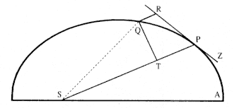
Figure 10.1
Based on Newton's diagram for Proposition 6 of the 1687
Principia .

The Orbital Equation and Curvature

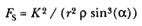
The polar orbital equation can be written in an alternate form as the curvature orbital equation, F_r = K ² / (r²r sin³ (a )), where r is the radius of curvature and a is the angle between the tangent to the curve and the radius r . The demonstration of the equivalence of the two equations is based upon three analytical elements: Newton's demonstration of Kepler's area law, Newton's circular approximation, and Newton's original work on curvature.

The first relationship is an expression of Newton's Proposition 1, Kepler's law of equal areas in equal times. Figure 10.1 is based upon the diagram for Proposition 6 in the 1687 edition of the Principia . The general curve is APQ , the tangent to the curve is ZPR , and the center of force is S . The area A of the triangle SPQ is equal to (1/2) SP × QT , or what is equivalent, (1/2) SP × PR sin (a ), where a is the angle SPR between the radius SP and the tangent ZPR . If the radius SP is written as r and the tangential velocity at P as v , then in a given time Dt , the line segment PR is equal to vDt , and the area A is given by r vDt sin (a ). Thus, the rate at which twice the area A is swept out is given as follows:

where K is a constant proportional to the area swept out per unit time. This relationship is mathematically equivalent to the modern law of conservation of angular momentum, where K is the angular momentum per unit mass.

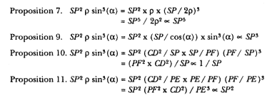
The second relationship is an expression of Newton's circular approximation: the replacement of motion along an incremental arc of the general curve at point P with uniform circular motion along an incremental arc of the circle of curvature at the same point. Figure 10.2 is based upon the diagram for Proposition 6 in the 1713 edition of the Principia . In his revised diagram, Newton added the normal to the tangent through the center of force YS and extended the line PS to the point V to display the

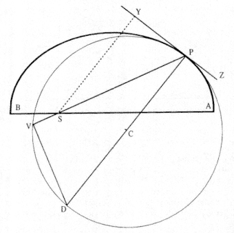
Figure 10.2
Based on Newton's diagram for Proposition 6 of the 1713
Principia .

chord of curvature through the center of force S . I have removed the points Q, R , and T , and I have explicitly displayed the circle of curvature PVD at the point P , where the center of the circle of curvature is at C and the diameter of curvature is PD (i.e., 2r ). The angle PVD between the chord and diameter of the circle is a right angle and a is the angle SPY (equal to the angle SPR in figure 10.1). The component of force F_C directed toward the center of curvature C is given by

where F_S is the force per unit mass directed toward the center of force S , and r is the radius of curvature. The force F_C directed toward the center of curvature C provides the centripetal circular acceleration v² / r as required in Proposition 4 of the Principia . Newton has explicitly employed this uniform circular replacement in Lemma 11, Corollary 3 and in Proposition 7, Corollary 5; and he has implicitly employed it in other discussions. Combining the two relationships, the force F_S directed toward the center of force S can be written as:

The third relationship concerns Newton's original work on curvature, which was extensive. It contains in detail what appears in the Principia only in outline. Central to the analysis is Newton's expression for the radius of curvature r in polar coordinates (r , q ), which he developed in the early 1670s. Newton expressed it in the following form:^[4]

where z' is dz /dq and z is the slope of the curve (1 / r ) (dr / dq ) = ctn (a ). It can be demonstrated that (1 + z² )^3/2 = sin^-3 (a ), where a is the angle between the radius r and the tangent to the curve, and that [(1 + z² ) – z' ] = r (r^-1 + d² (r ^-1 ) / dq² ).^[5] Thus, the expression for the radius of curvature r can be written also as follows:

If this expression is solved for (r^-1 + d ² (r^-1 ) / dq² ), then the polar orbital equation can be written in an alternate form as a function of r , r , and a : the curvature orbital equation.

The curvature orbital equation, expressed in terms of the radius r , the radius of curvature r , and the angle between the tangent and the radius a (i.e., F _r = K² / (r²r sin³ (a ))), echoes Newton's cryptic statement of 1664, in which he argued that the force (F_r ) for elliptical motion at a point (r ) can be found by the curvature (r ) at that point, if the motion (v and a ) at that point is given (i.e., F_S = v² / (r sin(a ))).^[6]

The Dynamics Ratios and the Orbital Equation

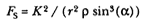
The linear dynamics ratio QR / (QT² × SP² ), which Newton derives in Proposition 6, is the functional equivalent of the contemporary orbital measure. Whiteside has demonstrated the relationship by expanding the geometric terms SP, QT , and QR in a power series, holding terms to the second order of the differential angle dq , and expressing them as a function of the analytic terms r , q , and their derivatives.^[7] It is also possible to use Lemma 11 to demonstrate the same result. Figure 10.3 is a revision of the diagram for Lemma 11 into the form that applies to Proposition 6. Lemma 11 states that AB² / BD = AG and if B approaches A , then AG approaches AJ , the diameter of the circle of curvature 2r . Written in terms of the elements of Proposition 6, AB ®QT / sin(a ), BD®QR × sin(a ), and AG ® 2r . Thus, the limiting value of the ratio AB² / BD is given by the following expression:

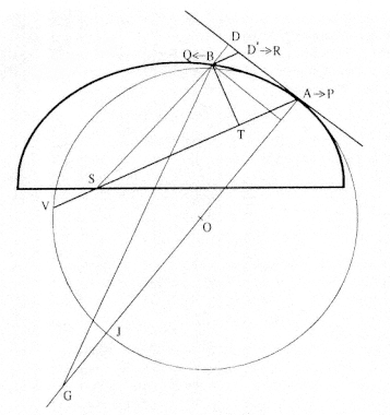
Figure 10.3
Newton's diagram for Lemma 11 adapted to the diagram for
Proposition 6.

which may be solved for the discriminate QR / QT² = 1 / (2r sin³ (a )). Thus, the linear dynamics ratio QR / (QT² × SP² ) is equal to twice the curvature orbital measure 1 / (r ²r sin³ (a )).

The circular dynamics ratio 1 / (SY² × PV ), which Newton introduced into the revised edition, also is identical with the curvature orbital measure. From figure 10.2 (given previously), the angle SPY is equal to the angle PDV or a (in fig. 10.2, both YS and PD are normal to the tangent YPZ and the angles PVD and YPD are right angles). The chord of the circle of curvature through the center of force PV is equal to PD sin(a ) or 2r sin(a ) and the normal to the tangent SY is equal to SP sin(a ) or r sin(a ). Thus, the circular dynamics ratio 1 / (SY² × PV ) also is equal to twice the curvature orbital measure 1 / [r²r sin³ (a )].^[8]

If the force is expressed in terms of the curvature orbital measure, then the solutions to the direct problems that Newton selected for the 1687 Principia fall into an interesting pattern.

For Propositions 7 and 9, the solution is simplicity itself because r and a are respectively constant. For both Propositions 10 and 11, however, one must note that the product PF² × CD² is proportional to the area of the ellipse, a constant, and for Proposition 11 that PE is equal to the semi-major axis of the ellipse, also a constant.

The choice of the orbit and focal center for Proposition 11 in 1684 was dictated by the physical problem of the planets, but the choice of the other examples was arbitrary. They may have been suggested by the work on curvature, which Newton began as early as 1664.^[9] In his Methods of Series and Fluxions of 1671, Newton calculated the radius of curvature for a number of examples, including conic sections and spirals.^[10] Newton's statement of 1664 indicated that he intended to use his work on curvature to solve direct problems of orbital motion. Whatever method he had in mind when he made the statement in 1664, however, it may not have been in the form of the curvature orbital measure 1 / (r²r sin³ (a )), because that measure entails the area law, which Newton did not discover before 1679.

Michael Nauenberg has suggested that before the discovery of the area law Newton could have employed a numerical method based on curvature to evaluate orbits. Nauenberg demonstrates an iterative computational method to reproduce the figure for the orbit of a body subject to a constant central force such as Newton sent to Hooke in 1679.^[11] Moreover, Nauenberg suggests that Newton could have used the material in his 1671 Methods of Series and Fluxions to produce an analytical measure of the force, independent of the area law, to solve direct problems.^[12] There is no evidence that Newton actually carried out such calculations, but Nauenberg

argues that there is considerable circumstantial evidence. For example, in the same letter of 13 December 1679 in which Newton sent Hooke the drawing of an orbit obtained by a numerical method for a constant force, Newton also noted that if the force increased as the distance decreased, then the body may "by an infinite number of spiral revolutions descend continually till it cross the center."^[13] Nauenberg suggests that Newton knew that the reciprocal cube force generated the constant angle spiral (logarithmic spiral). He notes that Newton's observation of "an infinite number of spiral revolutions" into the center cannot be deduced from a numerical solution of orbital motion, because that technique can provide only a finite number of revolutions in approaching the center. Nauenberg also points to Newton's choice of the constant angle spiral produced by a reciprocal cube force directed to the pole of the spiral as an example in the Principia for both the spiral / pole direct problem in Proposition 9 and the reciprocal cube inverse problem in Proposition 31.

It is also noteworthy that later in the Principia , Newton uses as an example the 1 / r³ force law, rather than the physically more interesting 1 / r² case, to solve explicitly the inverse problem, given the force law obtain the orbit (Book One, Proposition 31, Corollary 3).^[14]

Nauenberg argues that Newton could have solved various direct problems before 1679, and he challenges the received opinion that Newton could not have done so until after his discovery of the area law in 1679. In addition to this new debate over a solution for the direct problem, there is a long-standing debate over the outline for a solution to the inverse problem that Newton added to the 1713 Principia and extended in 1726.

The Revision of Corollary 1 of Proposition 13

In Corollary 1 of Proposition 13 in the 1687 Principia . Newton assumed that the solutions to the conic/focus direct problems given in Proposition 11, 12, and 13 also constituted a solution to the reciprocal square inverse problem.

From the last three propositions it follows that if any body P should depart from position P along any straight line PR, with any velocity, and is at the same time acted upon by a centripetal force that is reciprocally proportional to the square of the distance from the center, [then ] this body will be moved in one of the sections of conics having a focus at the center of forces; and conversely .

This statement is an improvement over the initial version in On Motion sent to Halley in 1684, in which only the solution to the ellipse/focus direct problem was presented and the other two conic sections were not discussed. Nevertheless, even as it stands in the 1687 Principia , this statement is unsatisfactory, and was criticized by Johann Bernoulli before the publi-

cation of the 1713 Principia .^[15] Newton's solution to the direct problem of conic / focal motion in the "last three propositions" (i.e., Propositions 11, 12, and 13) does not by itself constitute a solution for the reciprocal square force inverse problem. As Whiteside puts it,

The hidden assumption here made that no curve other than a conic may, in an inverse-square force-field centered on S , satisfy all possibilities of motion at P wants—for all its manifest plausibility—an explicit, rigorous justification, and Newton was later fairly criticized by Johann Bernoulli for merely presupposing its truth without demonstration.^[16]

Newton himself recognized the need to justify his assumption in the 1687 Principia of a solution to the inverse problem. In 1709, as the revised edition of the Principia was being prepared, Newton wrote to his editor Roger Cotes and requested that he add the following statement to Corollary 1 of Proposition 13 (Newton added the words in brackets to the 1726 Principia ).

Corollary 1. And the contrary. For the focus, the point of contact, and the position of the tangent being given, a conic section may be described, which at that point shall have a given curvature. But the curvature is given from the given centripetal force [and the body's velocity]: and two orbits mutually touching one the other, cannot be described by the same centripetal force [and the same velocity] .^[17]

Newton intended this extension to serve as an outline for the solution to the inverse problem, and evidently it satisfied Johann Bernoulli, for in 1719 he wrote to Newton as follows:

Gladly I believe what you say about the addition to Corollary 1, Proposition 13, Book One of your incomparable work, the Principia , that this was certainly done before these disputes began, nor have I any doubts that the demonstration of the inverse proposition, which you have merely stated in the first edition of the work, was yours; I only said something against the form of that assertion, and wished that someone would give an analysis that led a priori to the truth of the inverse [proposition] and without supposing the direct [proposition] to be already known. This indeed, which I would not have said to your displeasure, I think was first put forward by me, at least so far as I know at present.^[18]

Whiteside argues that Newton could have employed a general polar curve with given curvature to produce a solution for the reciprocal square force inverse problem without assuming the solution to the conic/focal direct problem.^[19] Newton did not, however, explicitly produce that solution (as he did for the reciprocal cube inverse problem in Proposition 31). Moreover, the validity of the outline of the solution of the inverse problem given in Corollary 1 of Proposition 13 in the 1726 Principia , which does assume the solution to the direct problem, continues to receive an occasional challenge. But now, as in the past, every challenger produces a number of

defenders. One recent challenger has claimed that Newton's solution, even as given in outline in the corollary, is radically flawed and contains a gross, irreparable fallacy. Another critic allowed that a gap may exist in the logic of Newton's outline, but argued that the gap is intuitively easy to fill. Other defenders argued that no gap of any sort exists.^[20] The Russian mathematician V. I. Arnol'd, however, saw no real basis for such a discussion. He argued, "The spirit of modern mathematics has penetrated to a number of physicists . . . and they have begun to worry about questions that earlier nobody would have talked about seriously." He arrives at the following conclusion:

In fact, all this argument is based on a profound delusion. Modern mathematicians actually distinguish existence theorems and uniqueness theorems for differential equations and even given examples of equations for which the existence theorem is satisfied but the uniqueness theorem is not. . . . Thus, in general, uniqueness does not follow from the existence of a solution, but everything will be in order if the solution produced depends smoothly on the initial condition. . . . For each initial condition [Proposition 17] Newton produced a solution, described it, and from this description it became obvious straight away that the solution depends smoothly on the initial condition. . . . Of course, one could raise the objection that Newton did not know this theorem. . . . But he certainly knew it in essence.^[21]

It is of interest to note that in the outlined solution of Corollary 1 of Proposition 13, as elsewhere in the Principia , Newton assumed on the part of the reader a background in the mathematics of curvature. In Lemma 11, the reference to curvature appeared only in a parenthetical expression, even though curvature was primary to the relationship developed in the lemma. In the final corollary to Proposition 7, the extension of the analysis on circular motion to the comparison theorem and general motion was defended by a final single sentence that called upon curvature. In Proposition 13, Newton again called upon his extensive work on curvature without an elaboration.

A Detailed Solution of the Inverse Problem

I now produce a solution to the inverse problem using Newton's equation for curvature that does not explicitly employ the solution to the direct problem (i.e., Propositions 11, 12, and 13).^[22] Instead, the solution employs Newton's work on curvature expressed in contemporary notation. There is no evidence that Newton actually produced such a solution for the inverse problem for gravitational force, but Whiteside argues that he was capable of doing so.^[23] The expression for the force obtained from the area law and the circular approximation is given by the curvature orbital equation as follows:

Newton's original expression for r = r (1 + z² )^3/2 / [(1 + z² ) – z '] can be expressed in terms of (1 + z² ) as follows:^[24]

Moreover, I have demonstrated that sin³ (a ) = (1 + z² )^3/2 . If r and sin(a ) are written in terms of (1 + z² ), then the expression for the force F_S can be rearranged and expressed as follows:

If the force F is given as c / r² , and (1 + z² ) is written as the function f (r ), then the equation reduces to:

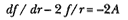
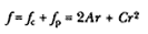
where A = c / K² . This equation is a first-order linear differential equation whose complementary solution f_c satisfies the equation df_c / dr – 2 f_c / r = 0 and is given by f_c = Cr² , where C is an arbitrary constant. The particular solution, f_p , is given by 2Ar , and thus the full solution f is:

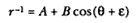
Substituting (1 + z² ) for f (as defined) and (B ² – A² ) for C (where B is arbitrary and A is given), and solving for z (defined as (r^-1 ) dr / dq ), the following relationship results:

Solving for the differential angle d q and integrating, one obtains the following relationship:

where e is a constant of integration. If that equation is solved for r ^-1 , then the polar equation of the general conic is given as follows:

Thus, as Newton argued in the statement he added to Proposition 13 in the revised Principia , the path is uniquely determined given the initial position and the curvature from the force and velocity.

Conclusion

Newton's contribution to dynamics must be measured not in terms of its correspondence with modern standards or modern methods, but rather in terms of the innovative and ingenious insights revealed in his initial

analysis. As early as 1665, and certainly before 1669, Newton had laid the foundations for his mature mathematical and dynamical analysis. Both the polygonal approximation and the parabolic approximation appeared in his pre-1669 analysis of uniform circular motion, and they were carried forward into his analysis of noncircular motion after 1679 following his demonstration of Kepler's area law. The circular approximation used in the alternate solutions of the 1713 Principia was based upon his work in 1664 on curvature. The solution to the direct Kepler problem, which is the hallmark of the 1687 Principia , had its roots in his statement of 1664.

If the body b moved in an Ellipsis then its force in each point (if its motion in that point bee given ) may bee found by a tangent circle of Equall crookednesse with that point of the Ellipsis .^[25]

That statement reached its fruition in the curvature orbital measure of force 1 /(r²r sin³ (a )), which has been demonstrated to be an alternate form of Newton's linear dynamics ratio of the 1687 Principia , his circular dynamics ratio of the 1713 Principia , and the modern polar orbital equation. If any single measure deserves the title of the key to Newton's dynamics, it is the curvature measure. To appreciate Newton's work on dynamics fully is to appreciate how it began in 1664 in the Waste Book , how it matured in the Principia , and how it relates to contemporary expressions of dynamics.