E. THE UNIVERSAL SCIENCE OF PROPORTION
The question of the quadratix and the kind of "line of proportions" its construction requires in fact puts us fight in the middle of the central problematic of Descartes's mathematics: proportionality. One of the main problems—one should probably call it the main problem—Descartes pursued throughout his career as a mathematician was the technique of constructing geometric proportionals. The construction of these proportionals had long been recognized as an issue in musical theory and was taken up in detail by the one author to whom Descartes acknowledges a debt in the Compendium, Gioseffo Zarlino.[30] The classic construction techniques of the ancient Greek mathematicians, employing ruler and compass, are in general not sufficient for producing an arbitrarily chosen number of geometric proportionals.[31] The mathematician Eratosthenes, however, took an important step in the development of more complicated, nonclassical devices for constructions by inventing the mesolabe, a set of interconnected triangles with pivoting arms that are able to slide in a rectangular framework. The mesolabe can be used to find two mean proportionals between two given line segments, which enabled Eratosthenes to duplicate the cube (i.e., to construct a cube double the size of a given cube). It also
[30] In Zarlino's Istituzioni harmoniche (Venice, 1558), 113-114, and Dimostrazioni harmoniche (Venice, 1571), 163-168; cited by Shea, Magic of Numbers and Motion, 38-40.
[31] Using just ruler and compass one can always find a point that determines a singte geometric mean proportional c between two lengths a and b. One can therefore also take this new line and find the mean proportionals between it and the other two (between a and c find d, between c and b find e ), thus acquiring three mean proportionals, d, c, and e, between the original lines; dividing each successive pair of these five lines yields four more mean proportionals, for a total of seven between the original two lines; dividing again produces a total of fifteen, etc. (i.e., one can use this technique to find l, 3, 7, 15, 31, 63, and in general 2 - 1 mean proportionals between the two original lengths). But one cannot in general construct an arbitrary number of geometric proportionals between two lengths. By contrast, for any counting number n one can divide the interval between two lines into n equal segments; that is, any arbitrary number of arithmetic mean proportionals can be found using ordinary techniques of construction.
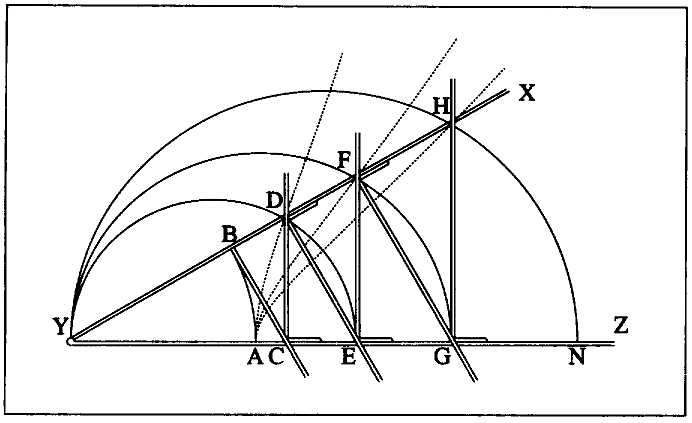
Fig. 5. Descartes's proportional compass. YX and YZ are joined by a pivot at Y; ruler BC (which can be made as long as necessary on side C) is rigidly attached to YX at a right angle; ruler CD has a sliding attachment that keeps it perpendicular to YZ; as do also EF and GH; similarly, DE and FG have sliding attachments to keep them perpendicular to YX. As the compass is pivoted open, the point of intersection between BC and YZ, that is, C, moves to the right, and the ruler BC pushes CD along YZ, CD pushes DE along YX, and so forth; when the compass is closed, all the rulers are pulled back toward Y.
can be used for dividing an octave into twelve equal semitones, for which purpose Zarlino mentions it.[32]
Apparently stimulated by the usefulness of the mesolabe, in early 1619 Descartes began to devise other mechanical instruments for solving complex geometrical problems. In particular, he made a geometrical compass that could in principle be used to find any number of geometric proportionals between two given lengths. The only limit was a practical one: how many rotating and sliding rulers could be manageably combined in a network of pivots and grooves. The construction of the instrument, pictured in figure 5, begins with two principal rulers, YX and YZ, pivoted at Y. These rulers are machined with grooves that allow the transverse rulers like BC
[32] After dividing the interval between a string and its midpoint into three geometrically proportional segments using the mesolabe, one then divides these three proportionally using just ruler and compasses (this produces six intervals between the original two lines), then divides each of these six again by a single proportional (yielding twelve intervals, the semitones of a musical octave).
and CD to slide as the compass is opened (that is, as angle XYZ is enlarged) or closed (XYZ gets smaller). These transverse rulers are attached in the following way.
First, BC is rigidly affixed to the upper ruler YX at B ; these two rulers always remain perpendicular to one another at this point. When XYZ is opened, point C will move progressively to the right along YZ . If we make rulers YX, YZ , and BC as long as we need and please, then as XYZ is opened very wide (so that YX and YZ are nearly perpendicular to one another) the point C will move toward the right to infinity, until finally BC becomes parallel to YZ when YX turns perpendicular to YZ.
So much for the first of the transverse rulers. The second transverse ruler, CD , represented in the figure as L-shaped, is fitted to the other rulers so that it will be pushed to the right by BC as the compass is opened and pulled back to the left as the compass is closed; as this happens, CD always remains perpendicular to YZ. Unlike the first transverse ruler, which is permanently attached at point B, CD and all the rest of the transverse rulers slide along either YX or YZ;C, D, E, F, G, and H are all moving points that move right or left according to whether the instrument is opened or closed, while the short leg of each transverse ruler keeps it perpendicular to either YX or YZ.
Thus the two principal rulers and the transverse rulers, as many as one likes (though here there are just six transverse rulers), are mechanically interlinked so that increasing or decreasing the principal angle XYZ causes the points C, D, E, and so on, to begin sliding; the transverse rulers push and pull one another into new positions as a network. For it all to function in a real instrument there would need to be appropriately tooled linkages: for example, a slot along the bottom of BC in which a button pivot attached to CD at C would slide as BC pushed or pulled on CD . In a similar fashion, DE will be attached to CD at D so that the ruler CD pushes or pulls DE to make the short leg of DE (at D ) slide along YX and the point E move to the right or the left along YZ. EF, FG, and GH will be attached and work in a similar way. With a routing tool and button pivots one could fairly easily construct a working version of such a compass. There is no limit in theory to the number of transverse rulers that can be used, but practically the instrument would soon grow bulky and stiff in its operation if one used too many.
The theoretical key to this compass's usefulness is that the interlocking rulers form triangles that are geometrically similar to one another. If one takes any two triangles formed by the various parts of the compass, one will find equal corresponding angles, and this assures that the lengths of the corresponding sides will maintain a strict proportion to one another. So, for example, in the triangles YBC and YFG , the angles at Y are equal, the right angles at B and F are equal, and the angles at C and G are equal;
therefore YB/YF = YC/YG = BC/FG. Triangle YBC is also similar to CBD, which is similar to DCE, which is similar to EDF , which is similar to FEG , which is similar to GFH ; YBC is similar to YCD, YEF , and YGH as well.
Because of these similarities we can set up a long series of proportions that hold between the ruler lengths. It is a simple exercise to see that HG/GF = GF/FE = FE/ED = ED/DC = DC/CB = CY/YB ; and even simpler that YB/YC = YC/YD = YD/YE = YE/YF = YF/YG = YG/YH. The compass is in effect a machine for generating series of line segments in constant, continuing proportion. So, for example, we can see that YC is the geometric mean proportional between YB and YD (since, from the beginning of the second equation string just given, YB/YC = YC/YD ; the geometric mean proportional between two numbers or lengths a and b is the number or length x such that a/x = x/b or, equivalently, such that x2 = ab ). YD is the geometric mean between YC and YE ; YE is the mean between YD and YF ; and so forth.
Now if we stipulate that YB is going to be our unit length, so that YB = l, we get 1/YC = YC/YD, which is equivalent to YD = YC2 . In the second equation string of the second sentence in the preceding paragraph, we have the equality YC/YD = YD/YE ; since we just showed that YD = YC 2 , we can substitute YC 2 for YD : YC/YC 2 = YC[2] /YE. Multiplying both sides of this equation by YC and by YE , then reducing it to simplest form, we get YE = YC[3] . Similarly, since YD / YE = YE / YF , we can substitute and work the equation to show that YF = YC[4] ; from YE/YF = YF/YG, we can reason that YG = YC[5] , and finally YF/YG = YG/YH lets us conclude that YH = YC 6 . If in theory or reality we build a compass with n transverse rulers, we can in a similar way find a line length that is equal to YCn for any positive integer n.
One of the things this compass does, then, is to raise the quantity c represented by the length YC to any power we like—or, more accurately, it raises it to all powers simultaneously, since YC, YD, YE, YF, YG, YH, and so on, represent the first, second, third, fourth, fifth, sixth, and so on, powers at the same time. Notice that to get all these powers one only needs to make YB the unit measure and open the compass until YC is of the desired length c ; one can then read the powers off of the principal rulers, with the lengths corresponding to odd-numbered powers lying along YZ and even-numbered powers along YX Inversely, one can take any number k , open the compass so that YD = k and have the square root represented by YC ; or open the compass so that YE = k and have YC be the cube root of k ; or open it until YF = k and have YC be the fourth (quartic) root of k ; and so forth. So the compass also extracts roots of any degree.
The last use of the compass to point out here—one that is a strict consequence of the preceding—is that it will display simultaneously any arbitrary number of geometric mean proportionals between two numbers/ lengths (presuming, of course, that we can add on transverse rulers at will).
Between YB and YG the compass displays the four mean proportionals YC, YD, YE , and YF ; between YB and YH it displays five (with YG added to the previous list). So given any two numbers a and b , set the scale on all the rulers so that YB = a (a scale, of course, just sets a basic proportion that will hold throughout all the terms of a problem or representation, as in a scale drawing),[33] expand the compass so that, say, YH = b , and one will have the five geometric mean proportionals.
Later, as is evidenced by the Geometry of 1637, Descartes continued his studies of this and related compasses, studies that were crucial for developing his version of what we call analytic geometry. The fundamental point is that if one takes YZ as fixed in place, it in effect becomes the equivalent of the x -axis of Cartesian coordinates in two dimensions, and the points of intersection between the transverse rulers and the upper principal ruler, that is, points B, D, F , and H , all trace out curves as the YX arm is rotated counterclockwise. These are the dotted lines of figure 5. Any such curve traced by the moving points of intersection of this compass is describable as an algebraic polynomial.[34]
In effect, these polynomial curves can be used geometrically to construct solutions to problems of proportion, even without the direct use of the compass. Contrariwise, the compass, with pencils attached to the moving points, can be used to trace polynomial curves. All the motions are rigidly interconnected and interdependent: the motion of any part of the device produces a determinate motion in every other part. This device and others like it, plus Descartes's researches into questions of how the procedures of sliding and rotating could be generalized mathematically to generate curves and figures for solving problems, are to be found in the last pages of the "Cogitationes privatae." For example, he conceives of a device for producing conic section curves by imagining a line capable of sliding through a fixed point while it simultaneously rotates around an axis; if the line is imagined to be a pen tracing out a curve on a fixed paper plane, the geometrical device becomes a practical one, an instrument for drawing conic sections. Such imagining provides the principle according to which a technician might devise corresponding practical machines. This technique of imagining the determinate configuration and motions of ideal machines occurs also in Descartes's work of the later 1620s, in particular in his search for devices to grind optical lenses.
Although we shall not follow these developments of Descartes's mathe-
[33] As we shall note presently, fixing the scale exactly, which is quivalent to determining he unit measure, is not always a solvable problem.
[34] An algebraic polynomial has the form a nx + an-1x + . . . + a2x + a1x + a0 , where n is a positive integer greater than or equal to o and all the terms aI are rational numbers (equivalently, one can restrict all the terms ai to integer values).
matics further, the crucial point is that Descartes's "analytic geometry" was derived from his examination of proportionality; it was driven by his discovery of an equivalence between (on the one hand) numerical/algebraic approaches and (on the other) geometric construction by the continuous, rigidly interlocked motions of mechanical instruments. Any algebraic problem, it seemed, could be embodied in a machine or compass, and any machine or compass could be used to generate what we would recognize as an algebraic polynomial in one unknown. These machines are perfectly describable by a mathematics using only rational numbers and therefore quite concretely and determinately imaginable.
At the end of the previous section and the beginning of this one, I mentioned a curve called the quadratrix. The quadratrix, Descartes realized, was the curve necessary for solving problems of compound interest. Its significance in the present context is that it cannot be generated by the kind of interlocking machines and compasses I have been describing. In figure 6, let OD and OC be our mutually perpendicular reference (coordinate) axes, fixed rigidly in place. Take a line segment OA and attach it by a pivot at O (this segment will rotate around O once we set the machine into operation). Take another line segment BC and attach it to OD so that it can slide up and down OD while remaining perpendicular to axis OD and parallel to axis OC . The machine will start working at time t0 with OA lying along OD and BC intersecting OD at A . We begin the motions by putting OA into clockwise rotation around O at a uniform speed and letting BC slide at a uniform speed downward along OD. We want to coordinate the rotation of OA and the downward slide of BC so that at the moment when BC reaches O (and therefore lies along OC ) the entire rotating segment OA will coincide with BC and OC . This device constructs the quadratrix as the line traced out by the moving point of intersection of OA and BG In figure 5, it is the curve marked by the points B, E, F, G, H . By attaching a pencil at this moving point of intersection we could actually draw the curve with an accuracy limited only by technical ingenuity.
What differentiates this "machine" from the proportional compass and other rigidly interlinked instruments is that it is not a single machine at all but two independent machines in need of coordination. The catch is that the coordination cannot take place by means of an interlinked system of pivots, sliding rulers, gears, or the like, connected in a way to assure that the two lines move uniformly and also coincide at exactly the right moment Such coordination can be achieved only approximately, and although there will always be ways to improve the approximation, it is impossible to give a solution that is general and exact.
With purely pragmatic goals supported by a sufficiently powerful technology, the lack of an ideal solution is a minor problem. One can still gain "control" over theoretical and practical problems apart from 100 percent
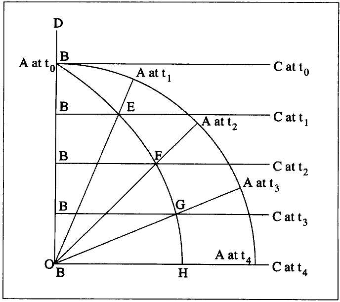
Fig. 6. Segment OA is pivoted at O and set rotating clockwise at a uniform rate; its positions at times t0 , t1 , t2 , t3 , and t4 are pictured. Simultaneously segment BC slides down axis OD at a uniform rate; its positions at times to through t4 are pictured. The two motions are coordinated so that OA falls along axis OC precisely at the moment (t4 ) when BC reaches it; at that moment OA, BC, and OC coincide. The quadratrix is the curve traced out by the moving point of intersection of OA and BC, indicated by the curve BEFGH.
accuracy and generality. The techniques of biplanar figuring would continue to be useful. But Descartes does not seem to have been interested in purely practical control without a theoretical certainty to back it up. The reasons are probably relatively simple. First, without knowledge of the exact solution, one cannot know how accurate a merely practical solution is. This is not to deny that in particular cases one can determine what the accurate solution would be: for example, there are simple techniques for constructing a limitless number of individual points of the quadratrix. Yet one loses thereby the economy that the general solution provides, and, even more important, one loses a careful and comprehensible understand-
ing of the relationships involved (i.e., one loses sight of the truth of the matter and its true cause or causes). In the solution of a single problem the resulting imprecision might matter little, but if the problem is part of a series of interconnected problems the uncertainties could quickly pile up in an indeterminate way, thus adding further uncertainties to any overall solution. Second, if a mechanical construction is impossible, the question arises whether this kind of motion is possible at all, that is, whether it could really occur in nature. God, of course, could bring it about, but not by ordinary, natural means.
Eventually, in the period leading up to the composition of the Geometry , the last of the essays accompanying the Discourse on the Method , Descartes became interested in the problem of systematically describing in algebraic terms the curves produced by the kinds of machines he had imagined in his youth. In the earlier period we can see traces of this interest, but it is not well developed. Although at the very end of the "Cogitationes privatae" he presents arguments about how algebraic equations of the fourth degree can be reduced to third-degree problems, he does not, surprisingly, call attention to any connections between his geometrical and his algebraic investigations. Their interrelationships are explicit in the Geometry , however; indeed, these interrelationships are its essential teaching.
Precisely when Descartes moved on to examine the essential structures of the interrelationship of algebra and geometric curves is a matter of debate. Looking at things from the longer perspective provided by the Geometry, one can nevertheless generalize: The kinds of machines Descartes conceived in the "Cogitationes privatae" can be used to trace out curves that are describable as analytic polynomials (i.e., curves that correspond to algebraic polynomials having whole number coefficients). In principle such curves are the result of raising a variable number (length) to a power (i.e., multiplying the variable length by itself the number of times indicated by the power, resulting in a "power length"), multiplying the result by a whole number (i.e., adding the power length to itself a whole number of times), and finally adding to or subtracting from one another all the resulting terms (lengths).[35] As a result, there is a translatability from a variable geometry into analytic polynomials and back, a translatability that provides powerful techniques for mathematical problem solving. A simple example: to solve an equation like x[5] = 4 one can in effect find four geometrical mean proportionals between a line of length 1 and another of length 4; contrariwise, to find solutions to geometrical problems, in particular those that require the construction of new line segments, one can translate the relationships into algebraic terms, perform successive
[35] As we shall see in chapter 3, this is the kind of mathematics presented in the uncompleted second part of the Regulae ad directionem ingenii.
operations on the equations to isolate the solution for an unknown, and then reproduce the geometrical analogs of these operations using geometrical figures and appropriate construction machines.
Things become more complicated when one allows irrational coefficients in the equations, that is, when the givens of the geometrical problem do not have a common measure, and more complicated still when the equations one is dealing with are no longer representable by a finite algebraic polynomial. The quadratrix is an example of the last, as are also the trigonometric functions (sines, cosines, tangents, etc.). One should realize, however, that the issue is not simply one of constructibility, since, for example, one can easily construct segments representing the trigonometric values for a given angle using just a ruler and a compass; likewise one can find as many points of the quadratrix as one likes using just these simple tools. The issue is rather whether the whole curve can be smoothly, continuously constructed by a constant motion that embraces every possibility, not just for a finite number of values or even for a potentially infinite number selected one by one.
In the letter to Beeckman of 26 March 1619, Descartes explained the goal he was pursuing with these and related researches.
And assuredly, as I shall lay bare to you what I am laboring at, I do not desire to propound a Llullian Ars brevis but a completely new science, by which might be solved generally all questions that can be put forward in any genus of quantity, continuous as well as discrete. But each according to its nature: for, as in Arithmetic, some questions are solved by rational numbers, some only by surd [= irrational] numbers, others finally can indeed be imagined but not solved: so I hope that I shall demonstrate that, in continuous quantity, some problems can be solved with straight or circular lines alone; others cannot be solved except with curved lines, but which arise from one single motion, and therefore can be drawn by the new compasses, which I consider no less certain and Geometrical than the common ones with which circles are drawn; others, finally, cannot be solved except by means of curved lines generated by different motions that are not subordinated to one another, which are certainly only imaginary: such a [curved] line is the quadratrix, [which is] well known enough. And I think that nothing can be imagined that cannot be solved at least by these lines; but I hope that I shall demonstrate which questions can be solved in this way or that and not another: so that almost nothing will remain to be discovered in Geometry. The work is virtually infinite, and not for one person alone. [It is] incredibly ambitious; but I have glimpsed through the obscure chaos of this science some sort of light, by the help of which I think every darkness, however dense, can be dispelled. (AT X 156-158; my emphasis)
Descartes's hope, as he spells it out here, is born of having conceived a science of quantity more general than either geometry or arithmetic. The former deals in magnitudes like length, width, and volume, which can take
on any value whatever, the latter in number, which is in essence based on the discrete elements of order. As any Aristotelian might have observed, these are both species of quantity, of the "how much." Thus his object is to develop a kind of mathematics that deals not with one or the other but with quantity per se. In arithmetic, problems can be divided according to the kinds of numbers that arise: the simplest problems are solved by counting numbers and the results of the four basic arithmetic operations (division, in particular, gives rise to the rational numbers); the next level of complexity is in problems that require surds, that is, irrational numbers that result from the four basic operations plus the taking of roots of any degree; the last is imaginary only, by which Descartes means not imaginary numbers in the modern sense[36] but rather solutions that require numbers that cannot be directly expressed by either arithmetic or root-taking operations (and so cannot be derived from the motions of rigidly interconnected machines) but are nevertheless determinate. For example, calculating the circumference of a circle requires the use of a number, pi , which is neither rational nor surd, yet it is quite determinately imagined as the ratio of the circumference of a circle to its diameter.
The problem of proportions was at the center of the mathematics of Descartes in large part because it appeared to him the key to arriving at a general method of solving problems. The construction of proportions falls into a general scheme that divides problems into those that can be solved by arithmetic proportions (rational numbers), those that can be solved by geometrical proportions (analytic, which means the solutions can be represented by a polynomial having rational coefficients), and those that can only be imagined (having transcendental solutions) hut not generally or mechanically solved. The criterion here is that classes one and two are both constructible and imaginable, whereas class three is only imaginable.
It is sufficiently clear, then, that exploring the power and scope of imagination was at the root of Descartes's early mathematics and science. The fundamental categories of the science of quantity were determined in accordance with imaginability, both the kind that is mechanically constructible
[36] That is, by taking the square root of a negative number. Although Descartes is sometimes credited with having in this passage initiated the modern usage of 'imaginary number' (see Gino Loria, "L'Enigma del numeri immaginari attraverso i secoli," Scientia 21 (1917): 105), it is clear that he is not referring to square roots of negative numbers but indicating imaginable but mechanically unconstructible solutions. AT agrees that Descartes is not referring to modern imaginary numbers but then suggests that he is thinking of solutions to equations higher than degree four (AT X 157). This seems doubtful to me, since equations of degree five and higher do not produce solutions different in kind from equations of lower degree, though perhaps the practical difficulties of solving higher-degree equations led Descartes to suggest this third kind of quantity (general techniques for solving equations of the first four degrees had been invented by the middle of the sixteenth century, and it was discovered later that there can be no general techniques for degree five and higher).
and the looser kind that is picturable but not constructible. There is a corollary: The realm of the corporeal is only a special case of the imaginable; the imagination in its most general form is more capacious and more powerful than the world that is merely given. One can imaginatively conceive what cannot be corporeally implemented.