Two
Greenhouse Gases: Changing the Global Climate
Michael C. MacCracken
Observations of the various temperatures of nearby planets and geologic reconstructions of climates tens to hundreds of millions of years ago, in association with calculations of the visible and infrared radiative fluxes, clearly demonstrate the potential for significant climatic change as emissions from societal activities alter the composition of Earth's atmosphere. In seeking to estimate the extent of future change, we can gain general guidance from analogs drawn from study of past climates, from analytic and laboratory studies, and from the trends beginning to emerge from the recent record, but none of these approaches can provide reliable, highly resolved estimates of the complex and unprecedented changes that society has initiated. There is also no definitive and convincing measurement—except for awaiting the outcome of our great "geophysical experiment"—that can alone serve as the basis for predicting the future climate.
In the absence of such traditional approaches to addressing the coupled physics and chemistry questions posed by the complex atmosphere-ocean-land-biosphere system, we are forced to rely on development of numerical models that seek to emulate all of the important and interacting processes.[1]
MacCracken and Luther 1985a; Schlesinger 1988.
The most comprehensive of these models are known as general circulation models (GCMs), which attempt to represent the three-dimensional, time-dependent character of the atmosphere and/or oceans. Modeling of the global climate is a particularly difficult challenge because the time scales of interest vary from hours to centuries, and spatial scales from kilometers to global. Even these broad scales, however, do not encompass the complete range of scales of atmospheric and oceanic motions—so that even if we can model the scales of interest, we must parameterize the effects of the smaller and shorter scales. Thus, we are forced into constructing models that not only incorporate thelimitations in our understanding of large-scale processes but also approximate the effects of smaller-scale processes known to be important in a deterministic, if perhaps not in a statistical, sense.
It is an open question whether such theoretical constructs can provide a sufficiently convincing basis for implementing important policy decisions concerning fundamental aspects of societal development and living styles. Although it is not possible to establish that the models we construct are correct—until after the fact—it is essential, as a minimum, that the ability of the models to represent past and present climates be clearly demonstrated against a range of past and present climatic changes if the models are to be used as a basis for policy formulation.
Predicting Global-Scale Warming
The potential global average warming expected to result from an instantaneous and perpetual doubling of the atmospheric carbon dioxide concentration (or its radiative equivalent from increases in the concentrations of carbon dioxide, methane, nitrous oxide, chlorofluorocarbons, and other greenhouse gases) is a convenient measure of the climate's sensitivity to radiative perturbations. In such calculations, it is assumed that oceans need to be represented only in terms of the heat capacity of their upper (50 to 100 m), mixed layer, which mainly governs the seasonal cycle thermal inertia, rather than in their full complexity. This simplification dramatically reduces the computer time needed to achieve a new statistical-equilibrium climate. Although these equilibrium calculations are not expected to simulate realistically the climatic response to the steadily changing composition of the atmosphere, especially because they do not account for potential changes in ocean circulation, they do indicate the commitment that society is creating to future climatic change. In addition, projections of greenhouse gas emissions suggest that we may become committed to these climatic changes by some time around the middle of the next century (and are already committed to about half of the projected changes even if we could somehow completely stabilize the atmospheric composition at present concentrations).
Results from models developed somewhat independently at five leading climate-modeling centers (i.e., National Center for Atmospheric Research [NCAR], NOAA Geophysical Fluid Dynamics Laboratory [GFDL], NASA Goddard Institute for Space Studies [GISS], Oregon State University, and the United Kingdom Meteorological Office),[2]
See Washington and Meehl 1984; Manabe and Wetherald 1987; Hansen et al. 1984; Schlesinger and Zhao 1989; and Wilson and Mitchell 1987.
when used to make roughly comparable simulations, estimate that global average surface-air temperature will increase by about 3° to 5° C for a doubling of the CO2 concentration.[3]Schlesinger and Mitchell 1987.
These values tend to be in the upper half of the estimated sensitivity range of 1.5° to 4.5° C adopted by National Research Council panels starting about ten years ago.[4]Charney 1979; NRC 1983.
Model intercomparisonstudies suggest that the treatment of clouds is the major cause of differences among the models.[5]
Cess et al. 1989.
Variations in cloud properties, which are not now well treated, could also be important factors in altering the sensitivity estimates.[6]Ramanathan et al. 1989.
There are several reasons to suggest that this order of magnitude is roughly correct. A doubling of the CO2 concentration results in an increase in the net tropospheric-surface trapping of infrared radiation by about 4 to 5 W/m2 . A number of tests of the models have been carried out that examine model responses to a wide array of other perturbations, which help provide some assurance that models are behaving realistically. The models represent the seasonal variations in mid-latitude temperature, which are driven by solar radiation variations of ± 100 W/m2 about the mean, to within about 10 percent.[7]
Grotch 1988. W/m2 = watts per square meter. The peak overhead solar flux is about 1370 W/m2 at the top of the atmosphere; the global average over 24 hours at the top of the atmosphere is about 340 W/m2, about half of which passes through the atmosphere and clouds and is absorbed at the surface.
Several models have successfully simulated the evolution of climatic conditions since the last glacial maximum, which involved seasonal changes in mid-latitude solar insolation of up to ± 40 W/m2 as a result of changes in Earth's orbit.[8]COHMAP 1988.
The models also do not exhibit an excessive sensitivity to the transitory perturbations of a few W/m2 caused by major volcanic aerosol injections, in agreement with the marginally detectable observed changes. Most recently, model results seem to be representing characteristics of the low-frequency climatic oscillations evidenced by the Southern Oscillation, the Quasi-biennial Oscillation, and other natural features.[9]E.g., Sperber et al. 1987.
Thus, although various processes in the models may not yet be fully and adequately represented, the model results provide strong evidence that the climatic sensitivity to a CO2 doubling will be a few degrees, not tenths of a degree or ten degrees.[10]
MacCracken and Luther 1985a.
Soviet reconstructions of climatic conditions tens of millions of years ago, when the natural CO2 concentration is believed to have been two to five times current levels, also suggest such a sensitivity.[11]E.g., Budyko and Sedunov 1988; Borzenkova 1988.
Predicting Regional-Scale Changes
Given the ranges of local temperature variations, a global-scale warming of a few degrees may seem a small price to pay for the benefits of energy, agriculture, refrigeration, and transportation. There is thus interest in determining the prospective changes with more spatial and temporal detail in order to be better able to evaluate potential impacts.
All model results indicate that the warming will be somewhat greater in high latitudes as the freeze season shortens and the warm season lengthens, the warming being amplified as the insulating effect of sea ice is reduced.[12]
Manabe and Stouffer 1980.
Paleoclimatic studies also indicate greater temperature changes in high latitudes than in low latitudes.On finer scales, the limitations of present models make estimation of regional scale climatic changes problematic. The horizontal resolution
of currently available general circulation models is typically five degrees of latitude and longitude (roughly 550 kilometers at the equator). In mid-latitudes, this resolution provides one grid point (with one value of temperature, wind speed, precipitation, etc.) for an area roughly the size of Colorado; in northern California, one grid point represents the diverse region extending from the Pacific Ocean west of San Francisco across the San Joaquin Valley and Sierra Nevada mountains into the deserts of Nevada.
Given such coarse resolution, developing an observation set against which to compare is not straightforward. Despite resulting limitations, when point-by-point comparisons are attempted, present models appear able to represent wintertime temperatures better than summertime, and larger scales better than smaller scales.[13]
Grotch 1988.
Over areas the size of the United States, differences between model results and observations of seasonal average temperatures are typically several degrees in summer, with deviations reaching up to 10° C in areas where the timing and extent of summertime drying are significant factors in determining surface temperature (e.g., the Midwest). Not only are treatments of hydrology in the models highly simplified (e.g., use of a fifteen-centimeter-deep "bucket" to represent soil moisture), but other assumptions in some models also make prediction of summer temperatures very difficult (e.g., no treatment of the diurnal cycle, poor treatment of nonraining clouds).Intermodel comparison of the estimates of the sensitivity of regional climatic conditions to a doubled CO2 concentration show very little spatial coherence, especially in summer and over land areas (see fig. 1). Although agreement among models does not assure that their results are correct, the low correlation coefficients among results from different models indicate that there is as yet no skill in predicting whether changes will be larger, for example, in the Southeast or in the Southwest. About all that model results indicate on a regional scale is that the local variations about the global average temperature changes will be strongly influenced by the balance between changes in precipitation (which will increase in many areas) and evaporation (which will almost certainly increase everywhere). Because models do not yet include comprehensive representations of the hydrologic cycle, however, the more or less random variation of results about the global average provides little useful indication of how precipitation may change. Improving this situation is a critical research objective.
Refining the horizontal resolution of the climate models is also expected to be necessary to improve simulation of regional climatic conditions significantly. There is a practical difficulty in accomplishing this, however; each halving of the grid size requires about an order of magnitude increase in computer time (four times as many horizontal grid
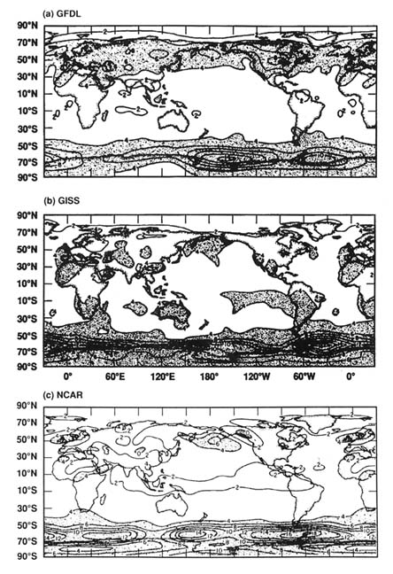
Figure 1. Geographical distribution of the surface-air temperature change
(°C), 2 × CO2 - 1 × CO2 , for June-July-August simulated with: (top) the
GFDL GCM by Manabe and Wetherald (1987); (middle) the GISS GCM
model by Hansen et al. (1984); (bottom) the NCAR GCM by Washington
and Meehl (1984). Stipple indicates temperature increases larger than 4° C.
points, twice the number of vertical grid points, and twice the number of time steps owing to the Courant instability condition, less not having to calculate some processes twice as often). Thus, fifty-year model simulations that now require a few hundred hours of supercomputer time would require a few thousand hours—making difficult significant testing of model parameterizations. A variety of other approaches to improving model resolution also merit consideration, including: refinement of the grid only in critical areas; driving a finer-grid mesoscale model with boundary conditions derived from a coarser-grid global model; using empirically derived relationships to go from large- to small-scale conditions (as is done in weather forecasting); or, perhaps, using more efficient computational techniques.
In addition to the computer demands required for greater resolution, a number of other factors also pose demands for increased computer time. Adding interactive chemistry to treat adequately the many interactions posed by the increases in chemically active trace gases could increase the number of prognostic equations from five to a few dozen.[14]
Ramanathan et al. 1985; Wuebbles and Edmonds 1988.
Interactively coupling atmosphere and ocean models, especially ocean models that have the fine resolution (e.g., 0.25° or finer) needed to resolve the important eddy motions and that represent the long time constants of the deep ocean, can increase computational requirements many times. Longer simulations are needed in order to treat cases with slowly increasing greenhouse gas concentrations. More accurately representing complex processes, such as hydrology, convection, and the land biosphere, will further increase computer demands.Another troubling feature of models concerns their ability to represent the full spectrum of variability seen in observations. Until recently it has appeared that model behavior is relatively stable, changing only slowly in response to external forcings, especially when the models do not fully couple the ocean to the atmosphere. There are, however, indications that past climatic conditions have changed relatively rapidly. For example, about a 0.3°C Northern Hemisphere warming occurred several times in the five years around 1920, and relatively sharp changes have occurred several times in the eighteen thousand years since the last glacial maximum. In the last several years, a few model calculations have exhibited either relatively rapid (i.e., decadal-scale) fluctuations, or even multiple equilibria.[15]
E.g., Hansen et al. 1988; Manabe and Stouffer 1988.
Inquiries into the potential for such surprise climatic shifts as well as into changes in the frequencies of short-term extreme events deserve greater attention.Projecting Time-Dependent Climate Change
Actual calculation of the rate at which climate should be changing requires a comprehensive atmosphere-ocean model that includes consideration
of the climatic effects of volcanic eruptions, solar variations, and the increasing concentrations of greenhouse gases since the preindustrial period and then into the future. There are not yet adequate models nor sufficient information fully to drive such models, although initial attempts are being made. For example, a calculation done at GISS using a simplified representation of the deep ocean, starting in the 1960s, shows a gradual warming that leads to global average temperatures exceeding maximum temperatures of the last interglacial period within the next few decades, depending on scenario assumptions about future changes in emissions.[16]
Hansen et al. 1988.
In lieu of complete calculations, an interpolation technique has been used to look at the consistency of model estimates of climate sensitivity and recent climatic change. Assuming the climate sensitivity to a doubling of the CO2 concentration (or equivalent through a radiative contribution by the several greenhouse gases) is actually a few degrees, then we would expect to observe a response as a consequence of the 25 percent increase in CO2 , the doubling of the CH4 concentration, and the increases in concentration of other trace gases above preindustrial levels. Dickinson and Cicerone (1986) estimate that the flux change from these combined changes is about 2.2 W/m2 , just half the 4.4 W/m2 they estimate would result from a doubling of the CO2 concentration. For a climate sensitivity range of 1.5° to 4.5°C for a CO2 doubling, this converts to a commitment to a temperature increase, at equilibrium, of about 0.75° to 2.25°C, based on the present atmospheric composition. There is currently considerable disagreement about the lag behind equilibrium caused by the time it takes to warm the oceans, with estimates from simple ocean models of the response time of the oceans ranging from a few decades to more than a century.[17]
Hoffert and Flannery 1985; Wigley and Schlesinger 1985; Hansen et al. 1988. An interesting corollary to the uncertainty in lag time concerns the associated thermal expansion of ocean waters and consequent sea-level rise. The long ocean lag times result when the oceans are assumed to be rapidly mixing heat from upper to lower layers; the short ocean lag times arise when deep ocean coupling is assumed to occur primarily as a result of polar bottom-water formation processes. When estimating potential sea-level rise out to the year 2100, the thermal expansion contribution to sea-level rise is about 2 to 3 times larger for the long ocean lag times for comparable climate sensitivities and emissions scenarios (e.g., 90 cm vs. 40 cm) (Frei, MacCracken, and Hoffert 1988). The sea-level rise over the past one hundred years has been 10 to 15 centimeters, presumably due both to thermal expansion and melting of mountain glaciers. Future sea-level change is also expected to result from both factors.
Accounting for this lag effect, the warming over the past 150 years would be expected to be perhaps 0.4° to 1.5°C.Many complications exist in attempts to compile estimates of global average surface-air temperature and other variables.[18]
MacCracken and Luther 1985b; Ellsaesser et al. 1986.
To provide a sufficiently lengthy record, resort is made to surface measurements of a wide variety of types, quality, and extent. Shortcomings exist because of changes in measurement method (e.g., canvas bucket to intake engine temperature for sea-surface temperatures), measurement locations and environment (e.g., the effects of urbanization), time of day of measurement, measurement accuracy (e.g., only to the nearest degree), varying spatial distribution of measurements, and many other factors. Despite these many difficulties with the data, better data would require upgrading the present multibillion-dollar global system for gathering weather data so that it could be more useful for monitoring the global climate. This would clearly be very expensive and require a commitment of many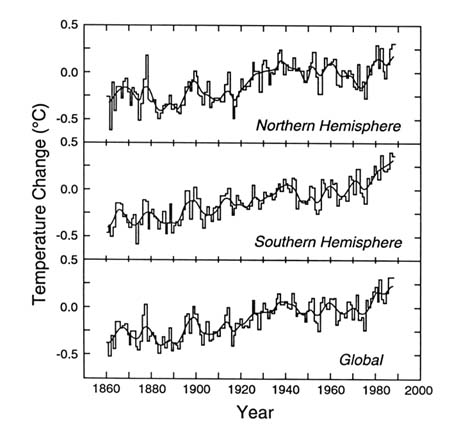
Figure 2. Area-weighted estimates of annual temperature departures from
a reference normal for the Northern Hemisphere, Southern Hemisphere, and global
land and ocean areas for the period since 1860. (Jones, Wigley, and Wright 1986)
years to provide a basis for examining climatic trends. At this time, we must therefore rely on what we have, despite the shortcomings.
Global compilations of available observations, which include a variety of approaches to account for possible data problems, suggest that average temperatures have increased about 0.5 ± 0.2°C since about 1850, as shown in figure 2.[19]
Jones, Wigley, and Wright 1986; Hansen and Lebedeff 1987.
Such a trend is seemingly in better agreement with the lower half of the NRC sensitivity range than the upper half that current model simulations appear to favor.Separate analyses of the Northern and Southern Hemisphere records also raise questions that must be answered to refine our understanding of the quantitative relationship between atmospheric composition and climate. The Northern Hemisphere record shows a cooling in the late
nineteenth century (probably due mainly to the climatic consequences of a series of major volcanic eruptions, but perhaps even a residual extension of the earlier Little Ice Age—a cool period during the seventeenth and eighteenth centuries, especially evident in land areas bordering the North Atlantic), a warming to the 1930s (particularly in high-latitude regions), a cooling into the 1970s, and a warming in the 1980s (mainly in low- and mid-latitude regions). Over rather large areas, particularly the eastern United States, cooling seems to have continued into the 1980s, keeping the average temperatures over the continental United States little changed this century.[20]
Karl, Baldwin, and Burgin 1988.
The cause of this irregular hemispheric warming may simply be natural variability or may also involve other perturbing factors. Possible examples include an increase in the anthropogenic sulfate aerosol loading causing an increase in cloud albedo (particularly in industrialized regions), volcanic aerosol injections, solar variability, ocean circulation changes, switching between possibly different circulation states, a nonlinear response to the CO2 /greenhouse forcing, or other factors.In the Southern Hemisphere the warming has been steadier and seemingly larger than in the Northern Hemisphere Given that the extensive land areas of the Northern Hemisphere have a lower heat capacity than the oceans of the Southern Hemisphere, that the warming is steadier in the Southern Hemisphere is not a surprise, but that it is larger is somewhat perplexing.
Taken together, the model simulations and the observed warming trend suggest that the potential global warming during the next century could well be several degrees but that our confidence is not better than a factor of two.
The Challenge To Society
The global environment is an essential resource for many if not all societal activities. Climate is an important influence on the environment, providing warmth and precipitation for agriculture and a suitable habitat for societal activities. Although the climate is not necessarily optimum in all areas, society has invested immense resources to adapt to present conditions (e.g., dams, aqueducts, buildings, etc.); thus, climatic change, especially if rapid or large, could induce significant stress, depending on the resilience and adaptability of the various activities. Even if slow, the likelihood is that small climatic changes, if continued and accumulated over a few centuries, could force significant alterations in the distributions of global population and of agricultural and forest areas.
An important complication arises because virtually all of the greenhouse gases, once injected, will remain in the atmosphere for decades to
centuries. The persistence of these compounds will lead to a new equilibrium climate. The oceans moderate the rate at which the climate approaches this new equilibrium and have thus allowed only some of the warming to occur to which we have become committed by past emissions. However, the ocean delay will not prevent the new, higher equilibrium temperature from eventually being reached. In addition, climatic effects will continue because emissions of already-produced gases (e.g., chlorofluorocarbons) have not yet all occurred, being slowed in many cases by temporary containment in foams and refrigeration equipment. Nor has the atmosphere come into a new chemical equilibrium with the released gases. Thus, even drastic actions at a given time (e.g., halting all new releases) cannot prevent further changes from occurring, although such actions could limit or moderate the amount of further change. The generation, use, and, ultimately, the emission of radiatively and chemically active gases occur, in almost every case, as a consequence of seemingly beneficial and essential (at least in narrow economic terms) societal activities, including provision of food, fiber, lighting, refrigeration, insulation, home heating, transportation, and medical services. The pervasive role of these gases means that controls and alternatives must be comprehensive and global in character; as a result, changes could be costly and slowed by the extensive effort needed to find alternatives and introduce replacements. Arbitrary or abrupt changes in the availability of such benefits could significantly affect the present standard of living in many areas.
The underlying challenge is for industrialized society to achieve a balanced and sustainable coexistence with the environment, one that permits use of the environment as a resource, but in a way that preserves its vitality and richness for future generations. Meeting this challenge will require development of an approach that, although recognizing the still tentative nature of the findings, encourages the countries of the world with their varying interests and concerns to respond in a timely and coordinated way. It will not be easy to minimize projected long-term environmental and societal disruptions while retaining the potential for nations, particularly the less well developed, to continue to improve their standards of living. But the challenge to transform our ways before our world is irrevocably changed could go far toward displacing militarization and the ever-increasing push for greater national consumption as the primary driving forces behind industrial activity.
Conclusions
Model calculations, supported by paleoclimatic and analytic studies and verified against a variety of cases of past climatic change, suggest that
the global average surface-air temperatures will increase several degrees during the next century if the increasing rates of emission of greenhouse gases continue. Such an increase would raise the long-term global average temperatures to levels not experienced in mid-latitudes back at least as far as the last interglacial period 125,000 years ago—and the change would occur more rapidly than ecosystems have been able to adapt to such changes in the past. Model projections of low-latitude temperature increases of a few degrees would raise temperatures to levels not experienced in tens of millions of years. (That the models indicate such high sensitivity in low latitudes, however, may be an indication that models are missing an important temperature-stabilizing mechanism that has been hidden because the observed seasonal variation in temperatures in these regions is so small.)
High-confidence predictions of global-scale temperature increases of such magnitude may provide sufficient information for the world to institute measures to slow the rate of increase of emissions and thereby the rate of temperature increase. Reducing total global emissions will be very difficult, however, without halting the increasing energy use and rising standard of living in the developing world.
Because continuation of at least present emissions levels seems highly probable, projections of potential changes at the regional level are needed to plan possible adaptive measures. Unfortunately, the reliability of the details of such forecasts is rather poor, so that decisions about whether a region must focus its response on increased winter precipitation or greater summer drying, or both, or neither, cannot yet be made. This does not mean that nothing can be done; rather it means that we must focus on increasing the flexibility and resilience of our activities that depend on the historic stability of the climate.
Thus, climate model results suggest that potential global environmental change may justify an ameliorative policy of reducing current emissions of man-made greenhouse gases but that expensive and comprehensive adaptive actions should generally await more certain results from improved models. While we labor at improving our models, we should also be identifying society's vulnerabilities to climatic change and setting in place programs to moderate potential impacts.[*]
Acknowledgment
This work was sponsored by the U.S. Department of Energy Atmospheric and Climate Research Division and performed by the Lawrence Livermore National Laboratory under Contract W-7405-ENG-48.
A more complete discussion of the policy implications of global warming and possible and appropriate policy options for the near term is contained in MacCracken 1990.
Notes
1. MacCracken and Luther 1985a; Schlesinger 1988.
2. See Washington and Meehl 1984; Manabe and Wetherald 1987; Hansen et al. 1984; Schlesinger and Zhao 1989; and Wilson and Mitchell 1987.
3. Schlesinger and Mitchell 1987.
4. Charney 1979; NRC 1983.
5. Cess et al. 1989.
6. Ramanathan et al. 1989.
7. Grotch 1988. W/m2 = watts per square meter. The peak overhead solar flux is about 1370 W/m2 at the top of the atmosphere; the global average over 24 hours at the top of the atmosphere is about 340 W/m2 , about half of which passes through the atmosphere and clouds and is absorbed at the surface.
8. COHMAP 1988.
9. E.g., Sperber et al. 1987.
10. MacCracken and Luther 1985a.
11. E.g., Budyko and Sedunov 1988; Borzenkova 1988.
12. Manabe and Stouffer 1980.
13. Grotch 1988.
14. Ramanathan et al. 1985; Wuebbles and Edmonds 1988.
15. E.g., Hansen et al. 1988; Manabe and Stouffer 1988.
16. Hansen et al. 1988.
17. Hoffert and Flannery 1985; Wigley and Schlesinger 1985; Hansen et al. 1988. An interesting corollary to the uncertainty in lag time concerns the associated thermal expansion of ocean waters and consequent sea-level rise. The long ocean lag times result when the oceans are assumed to be rapidly mixing heat from upper to lower layers; the short ocean lag times arise when deep ocean coupling is assumed to occur primarily as a result of polar bottom-water formation processes. When estimating potential sea-level rise out to the year 2100, the thermal expansion contribution to sea-level rise is about 2 to 3 times larger for the long ocean lag times for comparable climate sensitivities and emissions scenarios (e.g., 90 cm vs. 40 cm) (Frei, MacCracken, and Hoffert 1988). The sea-level rise over the past one hundred years has been 10 to 15 centimeters, presumably due both to thermal expansion and melting of mountain glaciers. Future sea-level change is also expected to result from both factors.
18. MacCracken and Luther 1985b; Ellsaesser et al. 1986.
19. Jones, Wigley, and Wright 1986; Hansen and Lebedeff 1987.
20. Karl, Baldwin, and Burgin 1988.
References
Borzenkova, I. I. 1988. Global climate sensitivity to the change of atmospheric gas composition from paleoclimatological data . Leningrad, USSR: State Hydrological Institute.
Budyko, M., and Yu. S. Sedunov. 1988. Anthropogenic climatic changes . Report prepared for the World Congress, Climate and Development, Climatic Change and Variability and Resulting Social, Economic and Technological Implications. Hamburg, 7–10 November 1988.
Cess, R. D., et al. 1989. Intercomparison and interpretation of cloud-climate feedback as produced by thirteen atmospheric general circulation models. Science 245:513–516.
Charney, J. 1979. Carbon dioxide and climate: A scientific assessment . Report of an
Ad Hoc Study Group on Carbon Dioxide and Climate, J. Charney, chairman, National Research Council. Washington, D.C.: National Academy of Sciences.
COHMAP Members. 1988. Climatic changes of the last 18,000 years: Observations and model simulations. Science 241:1043–1052.
Dickinson, R. E., and R. J. Cicerone. 1986. Future global warming from atmospheric trace gases. Nature 319:109–115.
Ellsaesser, H. W., M. C. MacCracken, J. J. Walton, and S. L. Grotch. 1986. Global climatic trends as revealed by the recorded data. Reviews of Geophysics and Space Physics 24:745–792.
Frei, A., M. C. MacCracken, and M. I. Hoffert. 1988. Eustatic sea level and CO2 . Northeastern Journal of Environmental Science 7, no. 1:91–96.
Grotch, S. L. 1988. Regional intercomparisons of general circulation model predictions and historical climate data . U.S. Department of Energy Report DOE/NBB-0084. Washington, D.C.
Hansen, J., and S. J. Lebedeff. 1987. Global trends of measured surface air temperature. J. Geophys. Research 92:13,345–13,372.
Hansen, J., et al. 1984. Climate sensitivity: Analysis of feedback mechanisms. In Climate processes and climate sensitivity , ed. J. E. Hansen and T. Takahashi. Washington, D.C.: American Geophysical Union.
Hansen, J., et al. 1988. Global climate changes as forecast by Goddard Institute for Space Studies three-dimensional model. J. Geophys. Research 93:9341-9364.
Hoffert, M. I., and B. P. Flannery. 1985. Model projections of the time-dependent response to increasing carbon dioxide . U.S. Department of Energy Report DOE/ER-0237. Washington, D.C.
Jones, P. D., T. M. L. Wigley, and P. B. Wright. 1986. Global temperature variations between 1861 and 1984. Nature 322: 430–434.
Karl, T., R. G. Baldwin, and M. G. Burgin. 1988. Time series of regional season averages of maximum, minimum, and average temperature, and diurnal temperature range across the United States: 1901–1984 . Historical Climatology Series 4–5. Asheville, N.C.: National Oceanic and Atmospheric Administration National Climatic Data Center.
MacCracken, M. C., and F. M. Luther, eds. 1985a. Projecting the climatic effects of increasing carbon dioxide . U.S. Department of Energy Report DOE/ER-0237. Washington, D.C.
MacCracken, M. C., and F. M. Luther, eds. 1985b. Detecting the climatic effects of increasing carbon dioxide . U.S. Department of Energy Report DOE/ER-0235. Washington, D.C.
MacCracken, Michael C. (Chair). 1990. Energy and climate change: Report of the DOE Math-Laboratory Climate Change Committee . Chelsea, Mich.: Lewis Publishers.
Manabe, S., and R. J. Stouffer. 1980. Sensitivity of a global climate model to an increase of CO2 concentration in the atmosphere. J. Geophys. Research 85:5529-5554.
Manabe, S., and R. J. Stouffer. 1988. Two stable equilibria of a coupled ocean-atmospheric model. J. of Climate 1:841–866.
Manabe S., and R. T. Wetherald. 1987. Large scale changes of soil wetness induced by an increase in atmospheric carbon dioxide. J. of Atmos. Sciences 44:1211-1235.
National Research Council (NRC). 1983. Changing climate . Report of the Carbon Dioxide Assessment Committee. Washington, D.C.: National Academy Press.
Ramanathan, V., R. D. Cess, E. F. Harrison, P. Minnis, B. R. Barkstrom, E. Ahmad, and D. Hartmann. 1989. Cloud-radiative forcing and climate: Results from the earth radiation budget experiment. Science 243:57–63.
Ramanathan, V., H. B. Singh, R. J. Cicerone, and J. T. Kiehl. 1985. Trace gas trends and their potential role in climate change. J. Geophys. Research 90:5547-5566.
Schlesinger, M. E., ed. 1988. Physically-based modeling and simulation of climate and climatic change, Parts 1 and 2 . NATO Advanced Science Institutes Series. Dordrecht: Kluwer Academic Publishers.
Schlesinger, M. E., and J. F. B. Mitchell. 1987. Climate model simulations of the equilibrium climatic response to increased carbon dioxide. Rev. of Geophysics 25:760–798.
Schlesinger, M. E., and Z. C. Zhao. 1989. Seasonal climatic changes induced by doubled CO2 as simulated by the OSU atmospheric GCM/mixed-layer ocean model. J. of Climate 2:459–495.
Sperber, K. R., S. Hameed, W. L. Gates, and G. L. Potter. 1987. Southern oscillation simulated in a global climate model. Nature 329:140–142.
Washington, W. M., and G. A. Meehl. 1984. Seasonal cycle experiment on the climate sensitivity due to a doubling of CO2 with an atmospheric general circulation model coupled to a simple mixed-layer ocean model. J. Geophys. Research 89:9475-9503.
Wigley, T. M. L., and M. E. Schlesinger. 1985. Analytical solution for the effect of increasing CO2 on global mean temperature. Nature 315:649–652.
Wilson, C. A., and J. F. B. Mitchell. 1987. A doubled CO2 climate sensitivity experiment with a global climate model including a simple ocean. J. Geophys. Research 92, no. 11:13,315–13,343.
Wuebbles, D. J., and J. Edmonds. 1988. A primer on greenhouse gases . U.S. Department of Energy Report DOE/NBB-0083. Washington, D.C.