Borrowing Strength

"Borrowing strength" is the colorful term John Tukey has introduced for the class of statistical procedures that seek to improve on naive estimates by incorporating data from parallel but formally distinct circumstances. These procedures also go under other names, such as pooling, random effects, James-Stein, shrinkage, empirical Bayes, and Bayes. The technique of damped regression provides an example most known to seismologists. Of the notion generally, Mallows and Tukey (1982) have remarked: "Knowing when to borrow and when not to borrow is one of the key aspects of statistical practice." A popular account of "improved" estimates is given in Efron and Morris (1977). The case of the linear model is developed, with examples, in Dempster et al. (1981).

To begin with a simple example, suppose that one wishes to estimate the mean µ_i of a population i , and one has available the mean

of a sample of

---

values from that population. Then the naive estimate of µ_i is

. Suppose, however, that other populations beyond the i th, and corresponding sample means, are available. Suppose that these populations are all somewhat similar. Let denote the mean of all the sample means of the populations. Consider borrowing strength, in the estimation of µ_i , from the other populations; specifically consider forming an estimate

for some q lying between 0 and 1. One would like to choose q to be near 1 if

can almost stand on its own, but q to be near 0 if the are highly variable. This problem may be formalized via a random effects model, specifically by setting down a model

with the Î_i , say, independent variates with mean 1 and variance t² , and the Î_ij independent variates with means o and variance s² . Then, for the case of samples all the same size, J , the "best" linear unbiased estimate of µ_i = µ + Î _i is given by expression (2) with

In the case that t is zero, q is 0, and the estimate is

. In the case that t is infinity, q is 1, and the estimate is .

As an example of what is involved here, consider the problem of developing attenuation relationships. Quite a variety of specific functional forms, involving a finite number of real-valued parameters, have been set down. For example, Joyner and Boore (1981) develop the relationship

for (mainly) western United States earthquakes with A peak horizontal acceleration, with M moment magnitude, and with d closest distance to the surface fault rupture in kilometers. To prevent earthquakes with many recordings from dominating the estimates, Joyner and Boore carried out the fitting in two stages. First magnitude was not included in the model, but an event constant was. Then the event constant estimates were regressed on magnitude to obtain the term – 1.02 + 0.249M. There were 23 events and 182 records in all.

One may obtain "improved" estimates as follows. The Joyner-Boore functional form will be retained. Let the subscript i index the event, and j index the record within the event. Consider the (random effects) model

where a_{i ,} b_ig_id_iI = 1, . . . , , are independent realizations of random variables with means m_a,m _bm_gm_d and variance

, respectively.

---

The Î_ij are independent noises with mean 0 and variance s² . This model ties together the events, but each event has its own a , b , g , d . (The usual nonlinear regression model corresponds to s_{a ,} s_b , s_g , s_d. identically 0.) Implications of this model are that records for the same event are correlated and that the disparate numbers of records for the events are handled automatically. Assuming that the random variables involved are normal, the model can be fit by maximum likelihood (employing numerical quadrature as needed). The results are provided in table 1. In some cases, for example s_a, s_d there is a clear suggestion that the corresponding population parameter may be 0.

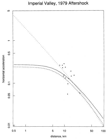
Once fit, model (3B) may be used, for example, for obtaining "improved" estimates of the attenuation behavior of the individual events. Consider for example the 1979 Imperial Valley aftershock. The data for this event are the points plotted in figure 3. Also plotted, as the curve of short dashes, is the result of fitting the Joyner-Boore functional form to the data for this event alone. Clearly, this curve is not too useful away from the cluster of observations. It has high uncertainty as well.

The solid curve graphed is the estimate of

with subscript 0 referring to this particular event. One has obtained a much more reasonable curve. This curve would be of use if one wished to estimate, a posteriori, an acceleration experienced in the Imperial Valley aftershock at a specified distance from the epicenter, for example to relate it to damage experienced at that distance.

The curve of long dashes in figure 3 is the Joyner-Boore curve, equation

---

Figure 3
Points plotted are observed accelerations at the indicated distances. The curve
of short dashes is the result of fitting the Joyner-Boore functional form to
these data points only. The curve of long dashes is the curve developed by
Joyner and Boore using the data set of twenty-three events. The solid curve
is the "improved" estimate developed from expression (4) and the model (3B).

---

(3A). It is not inappropriate. A thing to note however is that the Joyner-Boore curve is the same for all events of the same magnitude, here M₀ = 5.0. It does not take special note of the actual data for the event.

Figure 4 provides "improved" estimates for three other events. In each case, the improved estimates (solid curves) are plotted, as well as the Joyner-Boore (dashed) curves given by equation (3A). The general effect of borrowing strength here, and typically, has been to provide a curve lying nearer to the mass center of the points observed in the particular event of concern. Of particular note is the case of the 1957 Daly City event where but one observation was available. One could not sensibly fit a curve to that data point alone. The Joyner-Boore curve has some validity. The "improved" curve pulls the Joyner-Boore shape nearer to the available observation. In the case of the 1979 Imperial Valley event the two curves are very close to each other. This is the case with the most observations (38).