Possible Confounders in the Analysis of Birth-Order Differences in Intelligence

The analysis of birth-order differences in intelligence is not only beset by weak theory regarding the determinants of this presumed association, but it is also subject to weak theory concerning a large number of potential (and powerful) confounders when an apparent association is discovered. Although these confounders are not uniquely mysterious and arcane, they have frequently been overlooked because of the relatively casual and ad hoc approach to birth-order effects already noted in our discussion of predictors of birth-order differences. Investigators become interested in birth order when an "effect" turns up and happens to be startling. It is then relatively simple to weave an "explanation" out of some assortment of the advantages and disadvantages we have just discussed. It is seldom appreciated by researchers that expanding the sibsize distribution to a sibsize–birth-order matrix involves a level of specificity regarding, for example, the ages of parents and the periods of their lives during which particular children are born and reared that may be averaged out when one looks at sibsize alone.

It is hardly surprising, therefore, that research on birth order

and intelligence has produced perplexing disagreements concerning whether a birth-order effect exists and, if there is such an effect, what is its nature (for example, see, Jones 1931; Anastasi 1956; Sampson 1965; Adams 1972; Schooler 1972; Berbaum, Markus, and Zajonc 1982; Galbraith 1982a , 1982b , 1982c ; Ernst and Angst 1983). As we shall see, it is easy to be victimized by confounding factors, and exceptionally difficult, given the data available, to avoid all of them. As a start, we shall attempt to systematize some of the major confounding elements in the study of birth-order effects. A share of these confounders have been recognized in a scattered fashion in the literature, but some, I believe, have not been noted before.

Outline of Confounding Factors in the Analysis of Birth Order

1. The prevalence fallacy

2. Absence of controls for sibsize

3. Period effects

4. Parental background differences by birth order

5. Parental background differences by sibsize

6. Differences in child-spacing

7. Selection biases:

a. Age truncation biases

b. School-grade attrition biases (for example, seniors in high school do not include high school drop-outs who may differ from seniors in sibsize and birth order)

c. Other selection biases.

We may now consider each of these confounders in detail.

The Prevalence Fallacy

Probably the most obvious problem with some of the more striking findings on birth order is the bias introduced by looking at the proportionate prevalence of a particular birth order, or birth orders, in a selected group—for example, people of eminence or great talent, students taking a particular test, or those entering college at a particular time (for a discussion, see, Price and Hare 1969; Schooler 1972). All such research concludes that "x percent of persons who have a particular characteristic (eminent men, or

college entrants, or students having IQs of 140 or over) are of a given birth order (firstborn, last born, and so forth) and that, therefore, this birth order is highly desirable." Such prevalence studies with results sufficiently startling to report are subject to the bias of an excess of the birth order in question in the underlying population. Thus, to take college entrants in 1965, for example, a marked excess of firstborns is due to at least two major biases: On average, these students will be 18 years old and hence have a high probability of having been born in 1947—a year of the highest proportion of first-order births in our recorded past. Moreover, college students come from small families (disproportionately) and, hence, from families in which first-order births make up a high proportion of all births. So, not only will college entrants in 1965 share a disproportionate "firstborn-ness" with all 18-year-olds, but the small sibsize bias among middle- and upper-class young people will further potentiate the birth-order bias. As Schooler (and likewise Price and Hare) emphasize, the problems of bias in such prevalence studies remove all such "findings" from serious consideration.

From here on out, therefore, our discussion will relate to studies that involve the computation of values of a dependent variable by birth order and that compare the results for different birth orders. However, even when we thus avoid the prevalence fallacy, we are far from out of the woods regarding confounders.

Absence of Controls for Sibsize

As with many areas of scientific inquiry, knowledge is far from linear in birth-order research. Although it has long been recognized that, without a control for sibsize, birth-order effects will be confounded with sibsize effects (Jones 1931), this error continues to be made from time to time. For some recent examples, the reader may refer to Record, McKeown, and Edwards (1969) and King and Lillard (1983), in which sibsize effects are interpreted as birth-order effects.

Period Effects

The fact that children of different birth orders appear and are reared at different times in the parents' lives may mean that such children are subjected to markedly different economic and social

conditions as they mature. This may be particularly true for children from large families, but it can occur in small families as well during periods of rapid social and economic change. It seems reasonable to assume that such marked differences in environment might affect children through effects on their parents and on the latter's ability to provide a good learning environment. For example, if in 1968 one decides to study a sample of 18-year-olds, those from families of, say, six children will have experienced quite different periods in the U.S. economy depending on whether they are the oldest or the youngest. The oldest in one family, born in 1950, will come from a family that started its childbearing and childrearing during boom times economically—from 1950 onwards. But the youngest from another family—also born in 1950—will come from a family that started its childbearing and rearing around 1930—during the Depression. The following diagram may help to clarify this point.

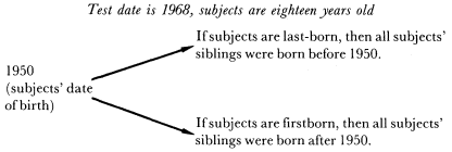
On the one hand, the confounding effects of a specific period are, of course, exaggerated in studies where individuals of only one age (or a very narrow age range) have been included—age truncation bias—since everyone has been subjected to the same historial event (being of the same age and the same cohort). On the other hand, the period effects are easier to isolate (once the investigator is aware of them) when the age range of the subjects is narrower. Nonetheless, the exact pinpointing of period effects may be difficult unless one has fairly precise information on child-spacing and the interval between the parents' marriage and the birth of the first child.

A good example of what appear to be systematic period effects interpreted as birth-order effects may be found in the data from Breland's study of National Merit Scholarship Qualifying Test takers and Belmont and Marolla's data on young Dutch males

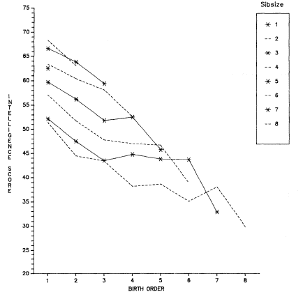
Figure 5.1.
T-Scores on Raven Progressive Matrices Test by Sibsize and Birth Order
among 386,114 19-Year-Old Dutch Males Who Were Survivors of Children
Born during 1944–1947. Data from Belmont and Marolla (1973). Scores
have been restandardized with a mean of 50 and standard deviation of 10.

(both of which have been referred to previously). Both studies show a marked decline in intellectual performance by birth order within sibsize (figs. 5.1 and 5.2).^[1] A share of this decline is doubtless due to differences in parental education by birth order (to be discussed shortly). In addition, the last-born children in the Dutch study suffered unique problems (also to be discussed). But, a share is also quite probably due to period effects to which both studies are particularly vulnerable since both concentrate on a highly restricted

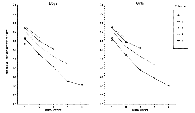
Figure 5.2.
T-Scores on National Merit Scholarship Qualifying Test by Sibsize and Birth Order among
794,589 Eleventh-Grade Boys and Girls, United States, 1965. Data from Breland (1974).
Scores have been restandardized with a mean of 50 and standard deviation of 10.

age grouping (17-year-olds in Breland's case and 19-year-olds in the Belmont and Marolla case). In fact, since the Breland youngsters were, on average, born in 1948, and the young Dutch men were born in 1944–1947, the economic period effects were similar. The oldest (firstborn) children were born to families that were beginning after the Depression, and as World War II was ending or over. On average, the families thus enjoyed improving circumstances as the youngsters were growing up. The later-born children (particularly those in large families) were born to parents whose reproduction started many years earlier—at the beginning of (or during) the Depression. Thus, most of the childbearing and rearing of the families of these later-born children occurred in unfavorable circumstances. It is unlikely that such circumstances left these families in a highly advantaged position to do well by their youngest children. Thus, as we see in figures 5.1 and 5.2, higher-order births do less well than lower-order ones—for period reasons among others.

Parental Background Differences by Birth Order within Sibsize and over All Sibsizes

The introduction of birth order as a variable necessitates controlling for differences in parental age (and, hence, most probably parental educational attainment) by birth order within sibsize. For example, in a group of 18-year-olds, all of whom are being studied in 1968, those who are the oldest of a family of six siblings were born to parents who started childbearing when the subject individual was born—1950. The youngest child in a family of six among these 18-year-olds was born to parents who completed childbearing in 1950, and who may have started it 20 years earlier, in 1930. Since, in most Western countries including the United States, educational levels of the population were rising over that time period, these young people's parents represent very different educational cohorts. If one does not control for the parents' educational levels among birth orders one may be simply measuring the effects, not of birth order, but of parents' educational differences within the same sibsize. Again, since parents' socioeconomic status was not controlled in either the Breland or the Belmont and Marolla data, the marked decline by birth order within sibsize of the intellectual scores would

appear to be in part a result of differential parental education—especially among children from large sibsizes. This differential may be added to the period effects already noted.

As has been noted previously, there are important parental background differences by sibsize. In looking at birth order, it is not sufficient to control for parental background differences by birth order within each sibsize; one has to control over all sibsizes as well. In other words, one must control for parental background differences among second-born children across all sibsizes containing such children, and the same is true of third-born, fourth-born, and so forth, rather than solely controlling for background differences between birth orders within each sibsize. If this is not done, the relative values by sibsize will be affected and, in particular, the position of the only child may be downgraded relative to children from other small families. The lack of controls for parental socioeconomic status over sibsizes in both the Breland and the Belmont and Marolla data may account for the unusual position of the only child in both studies, as we have already noted.

Differences in Child-Spacing

Theoretically, child-spacing differences may be confounded with birth-order differences, if systematically biased variations in child-spacing by birth order occur. For example, this confounding would take place if last-born children characteristically appeared after a longer interval than children of other birth orders. In practice, it seems unlikely that such systematic spacing differences by birth order would occur over large samples. This is particularly true for younger subjects in the United States since child-spacing itself has become much less variable than in the past. Infant mortality and breastfeeding (which created "spaces" in the past) have declined, and family planning has led to a purposive concentration of childbearing with a sharply defined ending point (Whelpton, Campbell, and Patterson 1966; U.S. Bureau of the Census 1976; Bumpass, Rindfuss, and Janosik 1978). Women have begun childbearing in their late teens and early twenties, and most have curtailed it before age 30. However, insofar as differential child-spacing does exist, certain kinds of samples may lead to systematic child-spacing effects that can show up as birth-order effects. This problem is evident in age-truncation biases to be discussed in the next section.

Selection Effects

We have already seen, with regard to the only child (considered as a sibsize), that selection effects can be important in affecting the relative position of children from a particular sibsize. We have also seen that selection effects, such as when seniors in high school are studied, can influence relative sibsize standings on IQ tests or National Merit Scholarship Qualifying Test findings. This is because less able young people in large families are more likely to have dropped out of high school than less able young people in small ones, and this differential drop-out rate has biased the IQ—sibsize relationship. Now we must consider how selection can affect birth-order findings.

The reader should consider this discussion to be illustrative only, since there are probably as many selection effects as there are research designs.

Age-truncation Biases

The problem of age truncation (sampling a single age or a very restricted age group) occurs quite frequently in birth-order research on intelligence because young people are being sampled. For example, if one has sampled 11-year-olds, those who are the oldest and from large families must come from closely spaced families because all of the children in the sibsize must have been born during an 11-year period. The youngest 11-year-olds from large families have not necessarily come from such closely spaced sibsizes. Thus, it is not at all uncommon to find that, among youthful samples, there may be an upturn for later-born children in the dependent variable (say, in IQ), an upturn that cannot be interpreted out of hand as a birth-order effect. The upturn at later birth orders in IQ testing is a not-infrequent result among age-restricted samples of young people, as figures 5.3 through 5.5 illustrate.^[2]

We should emphasize here that in general very wide spacing in large families (six or seven or more siblings) is not possible. For example, women beginning childbearing at age 20 and having a child every five years would be limited to five children even assuming that their last child was born when the woman was 40. It is thus not practical to think of wide spacing in families of six or seven or more as a generally compensatory mechanism allowing parents to provide more attention to each child—although obviously an individual child, or even two children, can be widely spaced in an

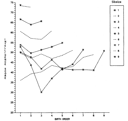
Figure 5.3.
T-Scores on Group Test of Intelligence by Sibsize and Birth Order
among Scottish School Children Age 11 in 1947. Data from the
Scottish Council for Research in Education (1949). Scores have been
restandardized with a mean of 50 and standard deviation of 10.

otherwise closely spaced family. Although extremes in spacing are uncommon, it would be desirable to know more about spacing in data sets such as we have been using because such information would provide an important test of the dilution hypothesis. Other things equal, we would expect widely spaced youngsters to have characteristics associated with smaller family size.

School-grade Attrition Biases

Just as youngsters from large sibsizes may be selected out of school at an early age, it is also not improbable that youngsters of particular birth orders may stay in school

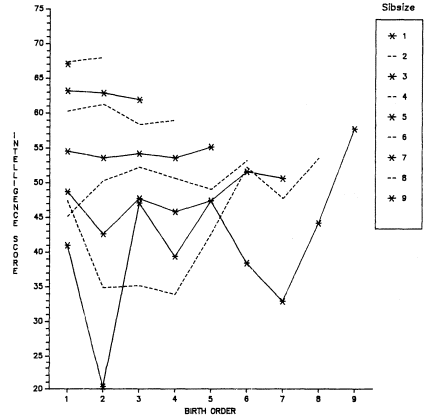
Figure 5.4.
T-Scores on Benedetto Test of Intelligence by Sibsize and Birth Order among
100,000 French School Children Age 6–14 in 1965. Data from Institut National
d'Etudes Demographiques (1973). Scores have been restandardized with
a mean of 50 and standard deviation of 10.

or drop out early, particularly in large families. For example, we shall see in a later section that, in large families, youngest and next-to-youngest children seem to stay in school the longest, whereas "early" middle-born children in such families (for example, third-born in families of six, seven, and eight or more) seem to be most deprived. It would appear, therefore, that sampling seniors in high school (and college students) for ability tests may well be selecting students from large families by birth order as well as by sibsize. Since last-born and later-born children appear to enjoy some economic advantages in large families (to be discussed), such

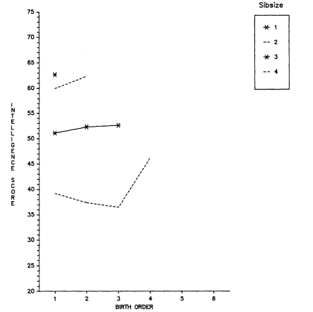
Figure 5.5.
T-Scores on Moray House Picture Test by Sibsize and Birth Order among
9523 Aberdeen School Children Age 7 in 1962. Data from Illsley (1967).
Scores have been restandardized with a mean of 50 and standard deviation of 10.

children may be less selected intellectually, other things equal, than earlier-born children in large families and, hence, on this count test less well as high school seniors (or college students) than youngsters from large families of other birth orders.

Other Selection Biases

The difficulty of distinguishing selection effects from birth-order effects is again illustrated from the Belmont and Marolla data on 19-year-old Dutchmen. As may be seen in

figure 5.1, not only do the results by birth order decline within each sibsize, but the last-born child in each sibsize takes a particularly sharp drop. The acute drop for each last-born child is quite different from the curves by birth order in any other data (figs. 5.2 through 5.5). It seems highly probable that this systematic drop in scores for all last-born children is related to the effects of the catastrophic famine in Holland during 1944 and 1945 (Smith 1947a and 1947b ; Stein and others 1972 and 1975; Blake 1981a ). In brief, since the famine drastically affected fertility, fetal mortality, and infant deaths, being an only child or other last-born child was a status that would occur selectively in those families worst hit by the famine (those families in which the woman could not become pregnant or stay pregnant to term or in which a next-born child would die). Moreover, since the adult death rate rose as well, many only and last-born children who were born during the 1944–1947 period, were partially or completely orphaned by the famine and, hence, remained "last-born." Again, on average this adult mortality would occur in those families worst affected by the famine. Since severe starvation in childhood is known to affect intellectual functioning adversely, it is hardly surprising that only and other last-born children in the Dutch data evidence an unexpectedly sharp drop in performance on the Raven Progressive Matrices test. The sharp drop among youngest children in the Dutch data led Zajonc (1976) to speculate that it was occasioned by a "teaching deficit." According to Zajonc, youngest children lagged intellectually because they (along with only children) had no siblings to whom they could act as mentors. In fact, I think it can be shown that this acute effect in the Dutch data is due to selection bias and that it is inadvisable to construct ad hoc substantive explanations for it.

To summarize our discussion so far, we have seen that theoretical expectations for birth-order differences in ability are weak and conflicting. We have no systematic, clear-cut reasons for expecting such effects. Moreover, when birth-order effects are found in empirical data, we have suggested that such effects are probably a consequence of one or more confounders—that the interpretation of effects as due to birth order may well be spurious. Different confounders will produce different "effects," and it is, therefore, hardly surprising that birth-order curves are so varied and difficult to interpret.

Before turning to our own empirical analysis of whether there

are birth-order differences in cognitive ability, we will consider in some detail the use, by Zajonc, of birth-order data to interpret the trend in SAT scores in the United States.