XIII. Dynamics of Ocean Currents
Our knowledge of the currents of the ocean would be very scanty if it were based entirely on direct observations, but, fortunately, conclusions as to currents can be drawn from the distribution of readily observed properties such as temperature and salinity. When drawing such conclusions, one must take into account the acting forces and apply the laws of hydrodynamics and thermodynamics as derived from theoretical considerations or from generalizations of experimental results.
For the sake of simplification, one may distinguish between four different methods of approach: (1) computations of currents from the distribution of density as obtained from observations of temperature and salinity, (2) conclusions as to currents caused by wind, (3) considerations of currents that result from differences in heating or cooling, precipitation or evaporation, (4) qualitative inferences as to currents which would account for special features of the observed distribution of such properties as temperature, salinity, and oxygen. Of these four methods of approach the first two are dynamical. The third involves considerations of a thermodynamical nature, and the fourth method is partly kinematic, but neither of these approaches is possible unless the dynamics of the system is understood.
The Hydrodynamic Equations
The Hydrodynamic Equations of Motion in a Fixed and in a Rotating Coordinate System. One of the fundamental laws of mechanics states that the acceleration of a body equals the sum of the forces per unit mass acting on the body. This law is applicable not only to individual bodies but also to every part of a fluid. The hydrodynamic equations of motion express only this simple principle, but, when dealing with a fluid, not only the equations of motion must be satisfied, but also the equation of continuity and the proper dynamic and kinematic boundary conditions.
The hydrodynamic equations of motion as developed by Euler take into account two forces only: an external force acting on a unit mass, and the total pressure gradients per unit mass. If the components of the

In this form or in the form obtained by substituting equation (XII, 17) for dv/dt, the equations represent the basis of classical hydrodynamics and have been used extensively for the study of many types of fluid motion. The only external force that needs to be considered in these cases is the acceleration of gravity. If the coordinate system is placed with the xy plane coinciding with a level surface, the equation takes an especially simple form, because the horizontal components of the external force vanish and the vertical is equal to g:
In many problems, friction must be considered, and to each equation a term must be added to represent the components of the frictional force.
The coordinate system used in these cases is rigidly connected with the earth and therefore takes part in the earth's rotation. When, for example, the flow through a pipe is analyzed, the x axis is placed in the direction of the pipe. This procedure is justified on the empirical basis that the observed motion can be correctly described in this manner. This fact, and only this fact, made possible the development of the Galileo-Newton mechanic. Phenomena exist, however, which cannot be adequately described by means of the simple equations of motion if accurate observations are made, as, for instance, the free fall of a body or the exact oscillation of a pendulum. In these cases the discrepancies between theory and observations are not very great, but for the large-scale motions of the atmosphere and the sea the discrepancies become so great that the simple equations fail completely.
The question arises as to whether it is possible to find another coordinate system in which the equations of motion in their simple form will describe the observed phenomena in an empirically correct manner. Experience has shown that this appears always to be possible. In the case that is of special interest here, it is found that the large-scale motion of the ocean waters can be dealt with if it is referred to a coordinate system, the center of which is placed at the center of the earth and the axes of which point toward fixed positions between the stars. Relative to this coordinate system the earth rotates once around its axis in twenty-four sidereal hours, and any coordinate system that is rigidly connected with the earth takes part in this rotation. The motion of a body on the earth relative to this “fixed” coordinate system is, as a rule, called the “absolute motion,” but incorrectly so because this “fixed” coordinate
It is impractical, however, to describe the currents of the sea in terms of “absolute” motion, for the interest centers around the velocities relative to the earth, and the problem is therefore to transform the simple equations of motion in such a manner that the new equations give the motion relative to a coordinate system that rotates with the earth. The transformation would require the development of equations which would otherwise not find use. The interested reader is therefore referred to the complete presentation by V. Bjerknes and collaborators (1933), from which part of the above explanation is taken. The transformation leads to the result that, if the equations of motion shall be valid in a coordinate system that rotates with the earth, it is necessary to add on the right-hand side of the equations the accelerations:

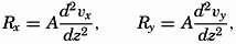
When applying the equations of motion to oceanographic problems, a left-handed coordinate system is used with the positive z axis directed downward. Taking this into account, adding the deflecting force of the earth's rotation, and including an as yet undetermined friction force with components per unit volume Rx, Ry, and Rz, one obtains the equations of motion in the form
The Deflecting Force of the Earth's Rotation. Many attempts have been made to show directly, without undertaking the complete transformation of the equation of motion, that the rotation of the coordinate system must be taken into account in the above manner. These
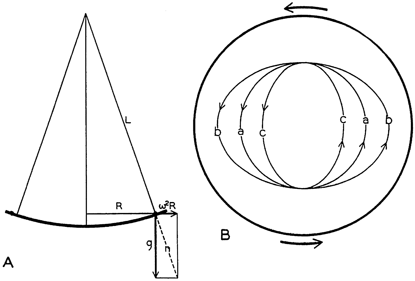
Motion of a body on a rotating disk. (A) Profile of the disk. (B) Different orbits of moving bodies.
Consider a disk that in an “absolute” system rotates at an angular velocity ω. Assume that a uniform gravitational force acts in the direction of the axis of rotation and that the disk has such a shape that the surface is normal to the resultant of the acceleration of gravity and the centrifugal force (fig. 101). Assume, furthermore, that the surface of the disk is absolutely smooth and offers no frictional resistance to any moving body. On these assumptions a body that rotates with the disk will complete one revolution in the time T = 2π/ω. A body that does not move in respect to an outside observer will, on the other hand, when placed on the disk, oscillate back and forth between two extreme distances from the center, R. The rotation of the disk does not affect this motion, since it has been assumed that the surface of the disk is frictionless. The period of the oscillation is easily found because in the first approximation the oscillation can be considered a pendulum motion (fig. 101). The period of oscillation of a pendulum is

Therefore, T′ = 2π/ω = T, where T is the time in which the disk completes one revolution.
If the observer gives the body a velocity equal to the velocity of the disk at the point at which he places it, the body will travel around with the disk and complete one revolution in the time T = 2π/ω. If the body is given a velocity greater or less than the velocity of the disk (fig. 101b or c), it will describe an ellipse in the same time T.
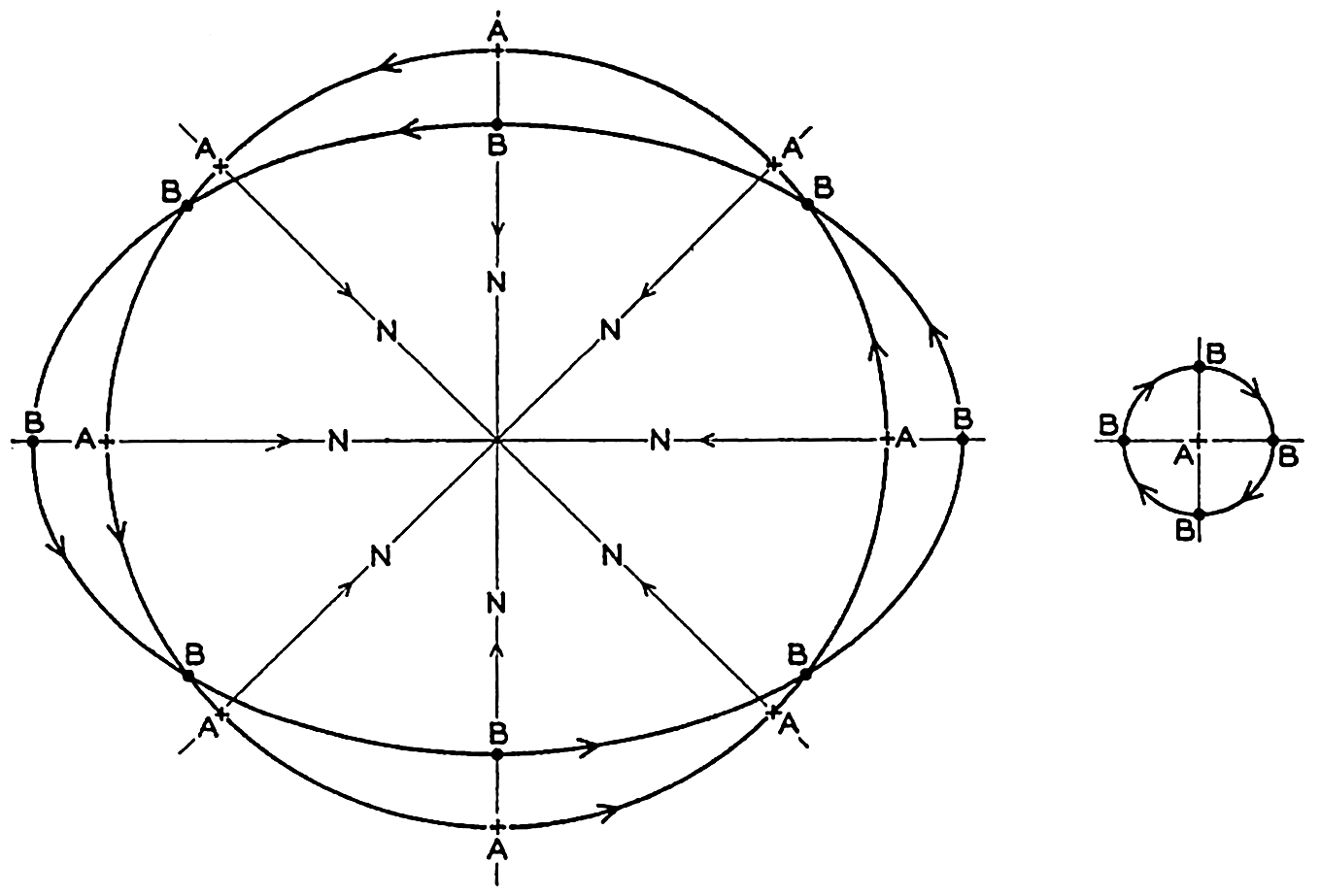
Motion of a body on a rotating disk as seen by an observer who looks down on the disk (left) or by an observer on the disk (right).
So far, the motion has been described relative to a fixed coordinate system. Now consider what an observer on the disk sees. This observer will refer the motion of the body to a coordinate system which, like himself, rotates with the disk and will, for instance, let the positive x axis point toward the center of the disk (fig. 102). Let the direction of the positive x axis be called north. Assume that the body at the time t = 0 was to the north of the observer and traveling faster than the disk. At the time t = T/8 the body will be to the east of the observer, at the time t = T/4 it will be to the south of the observer, at the time t = 3T/8 it will be to the west, and at the time t = T/2 it will again be to the north. To the observer it will therefore appear that the body travels in circles
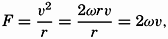
The apparent angular velocity of the body will be 2ω, and the linear velocity will be 2ωr, where r is the radius of the circle. In order to account for this motion the observer will say that a deflecting force directed toward the center of the circle exists which exactly balances the centrifugal force of the circular motion. The deflecting force must be equal to
The deflecting force performs no work, because it is always directed at right angles to the velocity. This conclusion is obvious, since the deflecting force is not a physical force but enters in the equations of motion only because the simple equations (XIII, 1) containing the physical forces have been transformed from the fixed coordinate system in which they are valid to a rotating coordinate system. It is a force, however, which, when dealing with relative motion, is just as necessary as any other force for a correct description of the motion, and which to an observer in the rotating system has the same “reality” as other forces.
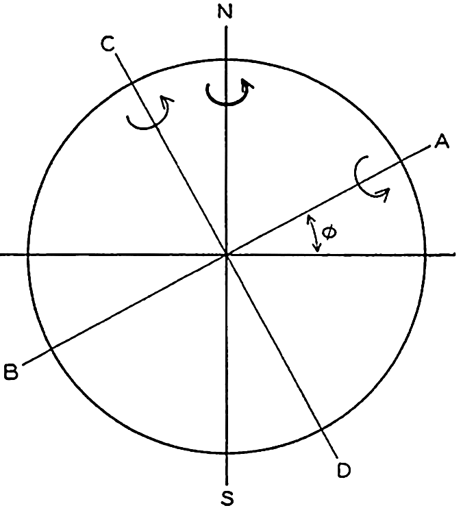
Rotation of the earth around the axis N-S decomposed in rotations around the axes A-B and C-D.
The above reasoning is directly applicable to conditions very near the poles of the earth, because a level surface on the earth is normal to the resultant of the force of gravitational attraction and the centrifugal force due to the earth's rotation.
In order to find what happens at a locality M at an angular distance of ϕ from the Equator (fig. 103), the rotation around the axis N-S can be considered as resulting from two rotations around the axes A-B and C-D. The angular velocities of rotation around these axes are ω sin ϕ and ω cos ϕ, respectively, if ω is the angular velocity of rotation around N-S. The rotation around C-D produces the vertical deflecting force
If no other forces are acting, the deflecting force must be balanced by a centrifugal force which, if the radius of the orbit is called r, is equal to ν2/r. Therefore
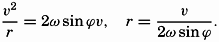
The radius of the orbit remains practically constant if the motion is such that variations in latitude are small, meaning that the particle will move in a circle of radius r. This circle is called the circle of inertia, because this circle, which appears in the relative motion, corresponds approximately to the straight-line inertia movement that characterizes “absolute” motion. In lat. 40° the radius of the circle of inertia is 106 m, 1060 m, and 10.6 km, respectively, if the velocity of the particle is 1 cm/sec, 10 cm/sec, or 100 cm/sec. The angular velocity of the body is 2ω sin ϕ, and the time required for one completion of the circle of inertia is therefore T′ = 2π/2ω sin ϕ. This time is called one half pendulum day, because it equals half the time required for a complete turning of the plane in which a pendulum swings (Foucault's experiment).
The motion in the circle of inertia in the Northern Hemisphere is clockwise, but in the Southern Hemisphere it is counterclockwise. In view of the fact that to an observer who faces the Equator the sun appears in the Northern Hemisphere to travel clockwise across the sky, and in the Southern Hemisphere counterclockwise, Ekman has introduced the term cum sole for describing the direction of motion in the inertia circle in both hemispheres. Similarly, the term contra solem describes rotation in the opposite direction.
It was stated that, when dealing with relative motion, the deflecting force is just as “real” as any other force. It can nevertheless be neglected when dealing with most problems of mechanics because, as a rule, it is very small compared to other forces. For instance, consider an automobile weighing 1500 kg which travels on a flat road in 40°N at constant speed of 75 km/hour (47 miles/hour) when the motor develops 15 kw (20.4 hp). The force per unit mass acting in the direction in which the car travels is then equal to 41.3 dynes/g. As the motion is steady, this force must be balanced by the resultant of the friction against the road and the deflecting force, but the deflecting force per unit mass, f = 2ω sin ϕ ν = 0.02 dyne/g, is less than 1/1000 of the other forces and can be neglected. The physical forces that maintain the motion of the atmosphere and the ocean, on the other hand, are of the same order of magnitude as the deflecting force, which therefore becomes of equal importance.
The effect of the rotation of the earth has been given so much consideration because in most problems the effect of the rotation enters and because the nature of the deflecting force should be thoroughly understood.
Motion in the Circle of Inertia. If the deflecting force of the earth's rotation is the only acting force, the equations of motion are reduced to

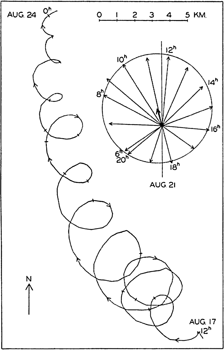
Rotating currents of period one-half pendulum day observed in the Baltic and represented by a progressive vector diagram for the period, Aug. 17 to Aug. 24, 1933, and by a central vector diagram between 6h and 20h on Aug. 21 (according to Gustafson and Kullenberg).
Gustafson and Kullenberg have represented the results of the records in the form of a “progressive vector diagram” (fig. 104), which is prepared
The curve shows a general motion toward the northwest and later toward the north, and superimposed upon this is a turning motion to the right, the amplitude of which first increases and later decreases. This rotation to the right (cum sole) is brought out by means of the inset central vector diagram in which the observed currents between 6h and 20h, August 21, are represented. The end points of the vectors fall nearly on a circle, as should be expected if the rotation is a phenomenon of inertia, but the center of the circle is displaced to the north-northwest, owing to the character of the mean motion.
The period of one rotation was fourteen hours, which corresponds closely to one half pendulum day, the length of which in the latitude of observation is 14h08m, and on an average the periodic motion was very nearly in a circle. It is possible that this superimposed motion can be ascribed to the effect of wind squalls and that the gradual reduction of the radius of the circle of inertia is due either to frictional influence or to a spreading of the original disturbance, but a theoretical examination by Defant suggests that inertia oscillations of this nature are associated with internal waves (p. 596). This was the case at the Altair station in lat. 44°33′N to the north of the Azores, where a rotating current of period 17h was present (Defant, 1940) corresponding very closely to a period of one half pendulum day and varying with depth in the manner found in internal waves. Ekman (1939) believes that the twenty-four-hour oscillations observed by himself and Helland-Hansen (1931) in about latitude 30°N are related to inertia movement.
The measurements that have been mentioned and other observations of currents made in deep water from anchored vessels (Defant, 1932, Lek, 1938) also show oscillating currents of tidal periods, some of which appear to be ordinary tidal currents, whereas others are associated with internal waves of tidal periods. In most instances, only tidal periods dominate and, according to Seiwell (1942), a period of one half pendulum day is not found in numerous oscillations which he has examined. It should perhaps be concluded that, although inertia movements may be found in the sea, it is still doubtful whether such a type of motion is very common. Arguments can be advanced against the general occurrence of movements in the inertia circle (Ekman, 1939).
The Equations of Motion Applied to the Ocean. When applying the equations of motion to the ocean, certain simplifications can be made. The vertical acceleration and the frictional term Rz can always be neglected. Similarly, the term depending upon the vertical component
At perfect hydrostatic equilibrium the isobaric surfaces coincide with level surfaces, but this is no longer the case if motion exists. At any given time an isobaric surface is defined by (p. 155)

Introducing the geopotential slope defined by iD,x = dD/dx, iD,y = dD/dy, and measuring the geopotential in dynamic meters, dD = gdz/10 (p. 403), one obtains
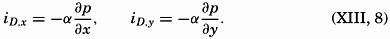
Thus, the geopotential slope in dynamic meters per meter equals the product of the specific volume and the pressure gradient in decibars per meter. These relations will find extensive use.
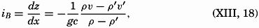
A dynamic boundary condition must be added to the kinematic boundary condition (p. 424)—namely, that at any boundary surface the pressure must be the same on both sides of the surface. This condition also applies to internal boundaries, separating water of different density, in which case the condition states only that the pressure must vary continuously. The densities and velocities may, however, vary abruptly when passing from one side of the boundary surface to the other. Calling the densities on both sides ρ and ρ′, and the velocities ν and ν′, and omitting the frictional terms and the accelerations, one obtains the dynamic boundary condition in the form

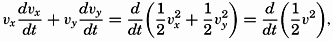
The dynamic energy equation is obtained by considering that the work done by a force is equal to the product of the force and the distance traveled in the direction of the force. Multiplying the equations of horizontal motion by νx and νy, respectively, and adding, one obtains

The equation is of small interest because it tells only that the increase of kinetic energy per unit volume equals the work performed per unit volume by the acting forces, but combined with the thermodynamic energy equation it becomes of importance. The complete derivation is given by V. Bjerknes and collaborators (1933), and here only the result for a system which is enclosed by solid boundaries is stated:

Here, W is the amount of heat added to the system, T is the total kinetic energy of the system, Φ is the potential, and E is the internal energy. If the total energy of the system remains unaltered, the amount of heat added in unit time must equal the work per unit time of the frictional forces. If, on the other hand, no heat is added, the work of the frictional forces must lead to a change of the total energy of the system.
Currents Related to the Field of Pressure
Relative Currents and Slope Currents. The above considerations are all general and are valid regardless of the character of the pressure field. When discussing the latter (p. 413) it was pointed out that the total pressure field could always be considered as composed of two parts: the relative field of pressure due to the field of mass, and the slope field due to actual piled-up masses: pt = p − Δp, where pt is the total pressure and p is the relative pressure, and where the last term represents a correction due to piled-up masses. With the pressure in decibars, Δp = gρΔh/10, where Δh represents the thickness of the removed or added mass in meters, and is positive when mass is removed, because the positive z axis is directed downward.
The total pressure gradient, therefore, has the components

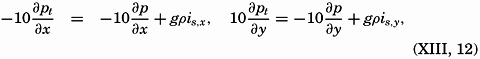
Introducing equation (XIII, 12) in the equation of motion, considering that pt has previously been written p, and omitting the frictional terms, one obtains
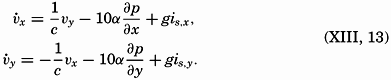
In the first approximation, therefore, writing νx = νp,x + νs,x and νy = νp,y + νs,y, one obtains
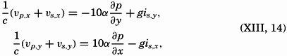
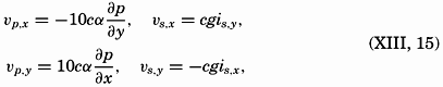
These equations mean that the current can be considered as composed of two parts: one which is dependent on the relative field of pressure and will be called the relative current, and one which depends on the added slope of the free surface and will be called the slope current. Ekman has called the relative current the convection current, but this term, as pointed out by Ekman, is liable to cause confusion because, in meteorology, convection currents mean ascending and descending currents and not horixontal flow.
Of these two types of currents, only the relative current can be derived from observations of density, because only the relative field of pressure can be determined from such observations. Any added slope of the isobaric surfaces due to actual piling up of mass in certain instances can be derived from precise leveling along coasts, but in general it cannot be observed. It is of great importance to bear these facts in mind in order to avoid erroneous conclusions.
The character of the slope current is readily seen. Equations (XIII, 15) state that the velocity is always directed at right angles cum sole relative to the slope. As the slope is independent of the depth, the same therefore applies to the velocity. Thus, if slope currents exist, they are uniform from top to bottom, in contrast to the relative currents, which vary with depth.
In the equations which, on the above assumptions, determine the relative current, the geometric or the geopotential slope of the relative isobaric surfaces can be introduced (p. 440):
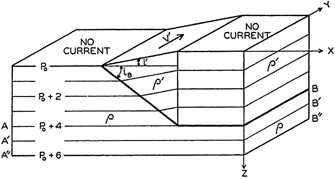
Currents in Stratified Water. Some of the outstanding relationships between the distribution of mass and the velocity field are brought out by considering two water masses of different density, ρ and ρ′, where ρ is greater than ρ′. In the absence of currents, the boundary surface between the two water masses is a level surface, the water mass of lesser density, ρ′, lying above the denser water. On the other hand, if the water of density ρ′ moves at a uniform velocity ν′ and the water of greater density moves at another uniform velocity ν, the boundary must slope. For the sake of simplicity it will be assumed that both water masses move in the direction of the y axis and that the acceleration of gravity g can be considered constant. The dynamic boundary condition (p. 441) then takes the form

As an extreme case, consider two water masses, one of salinity 34.00 ‰ and temperature 20°, and one of salinity 35.00‰ and temperature 10°, and assume that the velocity of the former is 0.5 m/sec. Neglecting the effect of pressure on density, one obtains

The slopes of the isobaric surfaces are much smaller. Inserting the numerical values in equation (XIII, 19), one obtains
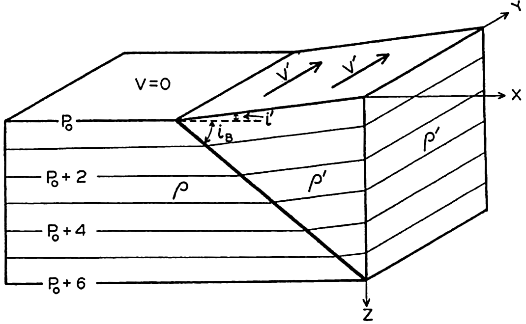
Isobaric surfaces and currents within a wedge of water which extends over resting water of greater density.
As another example, consider the case in which the current in the upper layer is limited to a band L. In this case, perfect static equilibrium must exist in the regions of no currents, and there the boundary between the two water masses must be horizontal, but in the region where the water of low density flows with a velocity ν′, the boundary surface must slope, the steepness of the slope being determined by equation (XIII, 18). These conditions are shown schematically by the block diagram in fig. 106, in which it is supposed that the denser water reaches the surface on the left-hand side of the current. This figure brings out an important relationship between the current and the distribution of mass: The current flows in such a direction that the water of low density is on the right-hand side of the current, and the water of high density is on the left-hand
Other examples could be added (Defant, 1929b), but the two which have been given here demonstrate sufficiently the relation between the currents and the distribution of mass in stratified water.
In the ocean a discontinuous transition from one type of water to another is never found, but in several regions a transition takes place in such a short distance that for practical purposes the layer of transition can be considered as a boundary surface. In such cases, equation (XIII, 18) can be used for computing the relative currents in a direction parallel to the boundary surface. Certain simplifications can be introduced, because ρ and ρ′ always differ so little that (ρν − ρ′ν′) can be replaced by  (ν − ν′). Therefore, the relative velocity can be computed by means of the equations

Isobaric surfaces and curreants within water which in part extends as a wedge over resting water of greater density.
The relative slope of the isobaric surfaces (XIII, 19) can also be expressed by means of the slope of a boundary layer:
The above equation can be derived in a different manner. In fig. 106, it has been assumed that the isobaric surfaces that lie completely in the

 . With this value, one obtains
 /L equals the slope of the boundary surface.
Where the isobaric surfaces slope, a current must flow in a direction at right angles to the slope, and with such velocity that the component of gravity acting along the slope is balanced by the deflecting force of the earth's rotation:
Currents in Water in Which the Density Increases Steadily with Depth. The discussion in the preceding paragraph leads directly to corresponding formulae in the general case in which the density of the water increases steadily with depth. The relative velocity has, as previously, the numerical value ν1 − ν2 = cgip1−p2, where ip1−p2 is the inclination of the isobaric surface p1 relative to the isobaric surface p2.
 and
and  (p. 408), the equation is reduced to

By means of the relations between the field of pressure and the field of mass, which were derived on p. 410, one similarly obtains (Werenskiold, 1937)


Equations (XIII, 26) are of practical importance because they facilitate a rapid survey of the relative currents at right angles to a section in which the field of mass has been represented by means of the anomalies, δ, or by means of σt curves. The inclination of a curve is positive when the curve slopes downward from left to right, because the positive z axis points downward (see fig. 107). Since “pressure”
In the Northern Hemisphere the current at one depth relative to the current at a greater depth flows away from the reader if, on an average, the δ or σt curves in a vertical section slope downward from left to right in the interval between the two depths, and toward the reader if the curves slope downward from right to left. In the Southern Hemisphere the current flows toward the reader if the curves slope downward from left to right, and away from the reader if the curves slope downward from right to left.
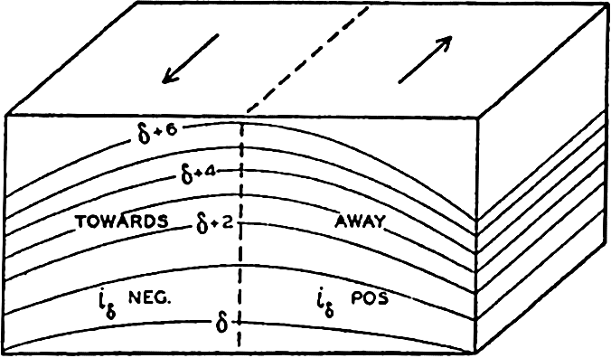
Schematic representation of a field of mass and of the direction of the currents which must be present if the field shall remain stationary (Northern Hemisphere).
These rules make possible an orientation as to the direction of the relative currents by a glance at a δ or σt section and a rapid computation of the approximate velocities.
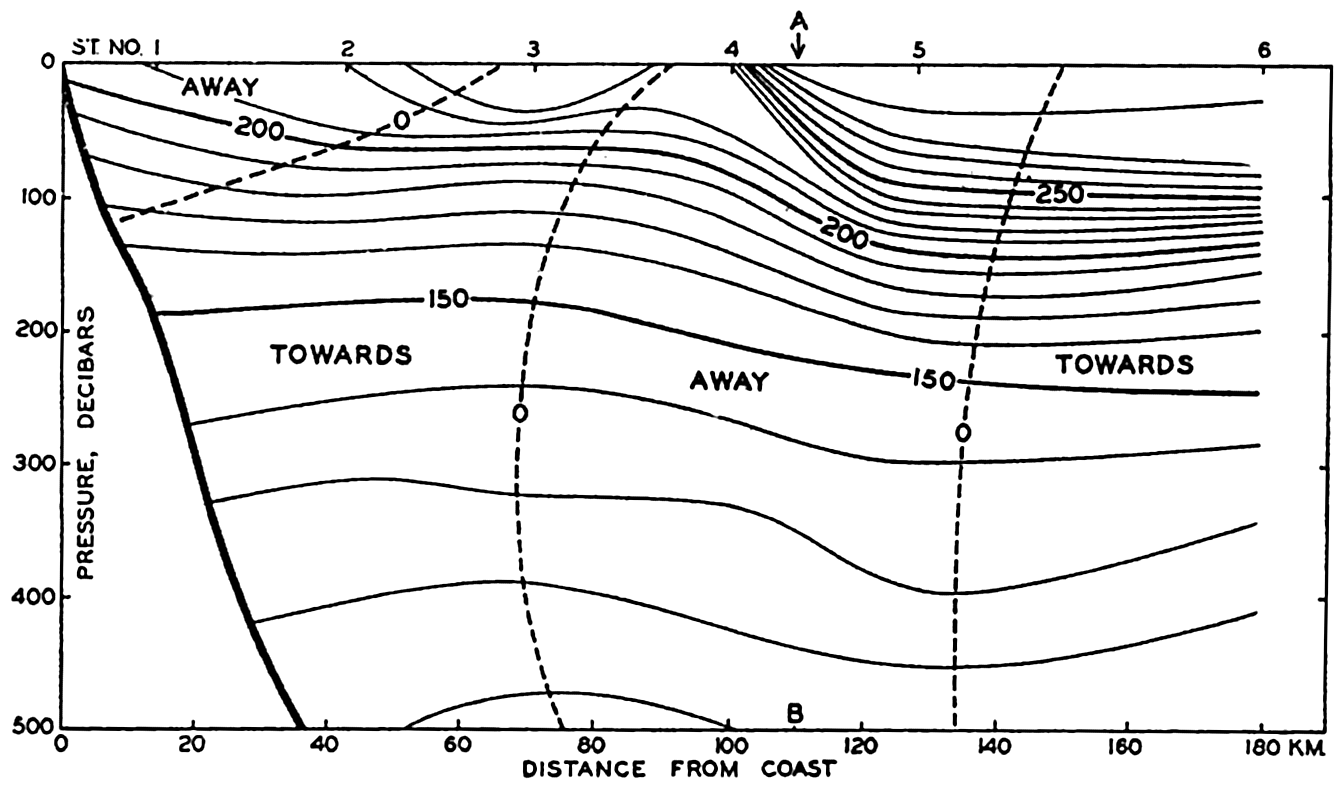
Specific volume anomalies in a vertical section at right angles to the coast of California in lat, 34.5°N, and direction of corresponding currents above 500 decibars.
Fig. 108 gives an example of a section at right angles to the coast of California in lat. 34.5°N. The section runs in the direction northeast-southwest, and the reader looks southeast. In the section, δ curves are entered at intervals of 10 × 10−5. The velocity relative to the
 is approximately zero between them and the 500-decibar surface. To the right the relative current is directed toward the reader, and to the left it is also directed toward the reader except within the upper layer. In the middle a strong current is directed away from the reader, toward the southeast. Along the line A-B,
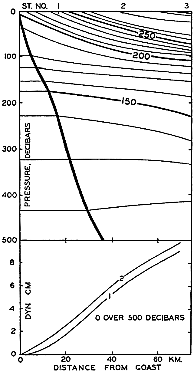
Upper. Specific volume anomalies in a vertical section at right angles to the coast of California in lat. 34.5°N. Lower. Profiles of sea surface computed (1) by continuing the anomaly curves horizontally from the point where they intersect the sea bottom, or (2) by assuming that the slope of the anomaly curves at the bottom determines the slope of the isobaric surface (see text).
Fig. 108 brings out a difficulty that is encountered when dealing with conditions in a section which extends into shallow water. In the figure the δ curves have been drawn to the solid line that represents the contour line of the bottom. Formula (XIII, 26), for computing the slope of the free surface relative to the slope of the 500-decibar surface, is applicable, however, only where the depth to the bottom is greater than 500 m, and loses its meaning if the depth to the bottom is less. The question then arises as to how the inclination of the free surface shall be computed when the depth to the bottom is less than the depth of the standard isobaric surface to which the inclination is referred. At the suggestion of Nansen, Helland-Hansen (1934) introduced a method which is actually based on the assumption that along the bottom both the
A similar method has been proposed by Jacobsen and Jensen (1926), but their formula introduces the additional assumptions that the profile of the bottom of the sea is a straight line and that the δ curves are parallel and at equal distances.
The assumption that the velocity vanishes at the bottom is probably always correct because of the influence of friction, but it is doubtful if the slope of the isobaric surface vanishes. As another approximation, one can apply the equation ip = − (δ1 − δ2) (p. 412), introducing the slope of the δ surfaces where they cut the bottom and taking the difference δ1 − δ2 along the bottom. In the lower part of fig. 109 the profile of the free surface is shown as computed by means of the two assumptions. The difference in this case is very small and, even under extreme conditions, will never be very significant.
No general rule can be given as to what method should be preferred. One may encounter conditions in which the assumption that the slope of the isobaric surface vanishes at the bottom is justified, and in such cases Helland-Hansen's method should be used, but in other instances, where it may appear improbable that the slope of the isobaric surface is zero near the bottom, the last-mentioned method should be preferred.
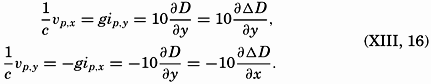
Practical Method for Computing Relative Currents. The formulae that have been dealt with in the last chapter are applicable to computation of currents at right angles to a vertical section. In order to derive a method for computing the currents in space, it is necessary only to return to equation (XIII, 16), which states that in the absence of friction and acceleration the velocity must be such that the deflecting force of the earth's rotation balances the component of gravity acting along an isobaric surface. It is now desirable to drop the assumption that the acceleration of gravity can be considered constant and to use the geopotential slope of isobaric surfaces instead of the geometric slope. It follows from equation (XIII, 16) that, on the assumptions made, the direction of the velocity will be normal to the slope of the isobaric surfaces—that is, parallel to the contour lines of the topography of the surfaces. The magnitude of the velocity will be inversely proportional to the distance between the contour lines, the factor of proportionality depending upon the latitude. The whole problem of presenting the
As has already been stated (p. 412), oceanographic observations can give information only as to the relative topographies, and therefore only as to the relative velocities. When using the term “relative velocity,” one should bear in mind that the absolute velocities (referred to the rotating earth) are not obtained by adding a constant value to the relative velocities, but that the value which has to be added in order to obtain the absolute velocities varies from one point to another, depending upon the unknown slope of the isobaric surface that has been used as a reference surface.
The contour lines of the isobaric surfaces represent the stream lines of the relative motion, but they are not, as a rule, identical with trajectories even if the reference surface is sufficiently level so that the computed velocities represent the absolute motion. If such is the case, the contour lines will be trajectories only if the motion is stationary—that is, if ∂ν/∂t = 0 (p. 157). Because it has been assumed that dv/dt = 0, it follows that the conditions
It is also of great importance to remember that equations (XIII, 16) and (XIII, 22) express nothing as to cause or effect. They do not state that the current is present because the distribution of mass is such and such. Nor do they state that the distribution of mass shows certain
The computation of the geopotential distances between isobaric surfaces has already been discussed, and the whole problem of computing ocean currents would therefore be very simple if (1) simultaneous observations of temperature and salinity at different depths were available from a number of stations so that relative topographies could be constructed, (2) accelerations could be neglected, (3) frictional forces could be neglected, and (4) periodic changes in the distribution of mass as related to internal waves (p. 601) were negligible.
Simultaneous observations from a number of stations are never available, and the question therefore arises as to whether charts based on stations that have been occupied within a certain time interval can be considered as approximately representing a synoptic situation. This question can be examined by repeated surveys of the same area. Such surveys have shown that conditions vary in time, but so slowly that the main features of a certain topography are represented correctly by nonsimultaneous observations that have been taken within a reasonably short time interval. Results of repeated surveys are found in the publications of the U. S. Coast Guard presenting the work of the International Ice Patrol off the Grand Banks of Newfoundland, where a small area has been covered in less than a week and where cruises have been repeated at intervals of three to four weeks. In these intervals of time the details of the relative topography have changed greatly, but the main features have changed much more slowly. Similar surveys have been conducted off southern California by the Scripps Institution of Oceanography (Sverdrup and staff, 1942).
Fig. 110 shows the results of two cruises off the coast of southern California in 1940. The upper chart shows the topography of the surface relative to the 500-decibar surface according to observations between April 4 and 14, and the lower chart shows the corresponding topography on April 22 to May 3. The stations upon which the charts are based are shown as dots. The time interval between the cruises was about sixteen days, and, although the main features were similar, the details were greatly changed. Thus, in lat. 33°40′N, long. 120°W, the computed surface current on the first cruise was 36 cm/sec toward N 80°E, whereas on the second cruise it was 14 cm/sec toward S 30°E. In the time interval between the two cruises the average local acceleration was therefore 2.5 × 10⁻⁵ cm/sec2 toward S 57°W, but, compared to the acting forces, this is a small quantity. On the first cruise the numerical value of the geopotential slope of the surface was 294 × 10−5 cm/sec2, and on the second it was 117 × 10−5 cm/sec2. The total acceleration is generally of the same order of magnitude as the local acceleration, and was therefore also small. Even in these cases the stream lines of the flow approximately coincided with the contour lines, although the distribution of mass was changing continuously, and the combination of observations taken during ten days led to a somewhat distorted picture of the topography.
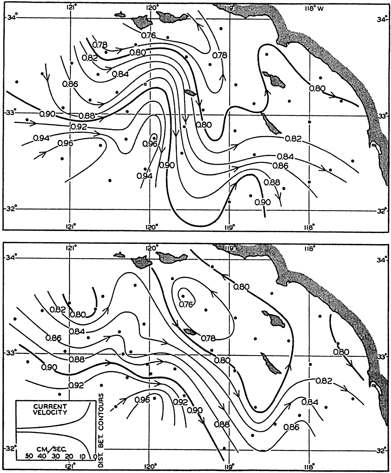
Geopotential topography of the sea surface in dynamic meters referred to the 500-decibar surface according to observations off southern California on April 4 to 14, 1940 (upper), and on April 22 to May 3, 1940 (lower).
As a rule, it can be stated that the smaller the area the more nearly simultaneous must observations be in order to permit conclusions as to currents. On the other hand, when dealing with ocean-wide conditions, observations from different years can be combined.
The second assumption, that the motion is not accelerated, is evidently not fulfilled when dealing with a smaller area within which conditions change rapidly, but, according to the above numerical example, no serious errors are introduced if one is satisfied with an approximate value of velocity. The assumption will be more closely correct when large-scale conditions are considered.
The third assumption, that the frictional forces can be disregarded, must also be approximately correct, as is evident from agreement obtained between computed surface currents and surface currents that are derived from ships' logs or from the results of experimentation with drift bottles. The fourth assumption is nearly correct where the accelerations are small. It can be stated therefore that the computations which have been outlined can be expected to render an approximately correct pictures of the relative velocities that are associated with the distribution of mass.
Absolute Currents Associated with the Field of Mass. In the discussion so far, we have considered only the relative currents associated with the relative field of pressure, but the ultimate goal must be to determine the absolute current. The problem of determining absolute currents can be dealt with in two steps. In the first place, one can consider whether there are reasons to assume that the absolute currents are determined completely by the internal distribution of mass. If this question is answered in the affirmative, one can decide what reference surface should be used in order to find the absolute motion.
The first question can be approached in the following manner: If the distribution of mass remains stationary, the flow must always be parallel to the isopycnals, because, if this condition is not fulfilled, the distribution of mass will be altered by the motion. On the assumptions made, the flow is always parallel to the isobars, and it follows, therefore, that under stationary conditions isopycnals and isobars must be parallel at all levels. It also follows that the isobars and isopycnals at one level must be parallel to those at all other levels (p. 157). This rule is identical with the “law of the parallel solenoids” of Helland-Hansen and Ekman (Ekman, 1923). The absolute motion that must be considered when dealing with distortion of the field of mass depends, however, on the total field, and this total field must evidently have the same geometrical shape as the internal field if the law of the parallel solenoid shall be fulfilled. The total field is composed of the internal and the slope fields (p. 413); consequently, these fields must coincide if the law of the parallel
The study of large-scale conditions in the ocean has shown that over large areas the isotherms and isohalines, and, consequently, the isopycnals, are parallel at different levels and that their direction coincides with the direction of the relative isobars or with the contour lines of the isobaric surfaces. This empirical result strongly supports the view that the large-scale currents are mainly determined by the internal distribution of mass. Even in small areas a similar arrangement is often found, but many exceptions are encountered there which clearly demonstrate that stationary conditions do not exist, and which may be interpreted as indicating that the details of the absolute currents are not determined by the distribution of mass.
The next question that arises is whether it is possible in the ocean to determine a surface along which the velocity is zero, so that absolute velocities are found when the relative motion is referred to this surface. Such a surface need not be an isobaric surface but may have any shape.
One school of oceanographers points out that the deep waters of the oceans are nearly uniform and that in the deep water the isopycnal surfaces are nearly horizontal. It is therefore assumed that in the deep water the isobaric surfaces are also nearly horizontal and that absolute currents are found if the reference level is placed at a sufficiently great depth.
A second school of oceanographers claims that the distribution of oxygen in the ocean must be closely related to the type of motion, and especially that the layer or layers of minimum oxygen content that are found over large areas must represent layers of minimum horizontal motion. Consumption of oxygen takes place at all levels, owing to biological processes, and it is reasoned that minimum oxygen content is found where the replenishment of oxygen by horizontal flow is at a minimum because of weak motion. Rossby (1936a) and Iselin (1936), among others, have drawn attention to the fact, which has been clearly demonstrated by Dietrich (1937a), that this conception may lead to peculiar results concerning the currents. In the Gulf Stream, with the 2000-decibar surface as reference surface, one finds flow in the direction of the Gulf Stream from the sea surface to a depth of 2000 m, whereas, by selecting the oxygen minimum layer as reference surface, one finds that the flow in the direction of the Gulf Stream is limited to the upper layers, while at greater depths the current flows in the opposite direction with velocities that increase toward the bottom. The latter type of flow appears unreasonable, and therefore the oxygen minimum layer in that case cannot be a layer of no motion.
Another argument may also be advanced against assigning dynamic significance to the oxygen minimum layer (Sverdrup, 1938a). As has already been stated with regard to this layer as a layer of minimum motion, it is argued that the low oxygen content is due to a slow replenishment of oxygen by horizontal flow. It must be borne in mind, however, that in the ocean the distribution of oxygen is nearly stationary, meaning that at any point the amount of oxygen which in a given time is brought into a given volume by physical processes, such as diffusion and horizontal flow, must exactly equal the amount which in the same time and volume is consumed because of biological processes. Therefore, if the oxygen minimum layer represents a layer of minimum replenishment, it must also represent a layer of minimum consumption, and this requirement leads to certain conceptions concerning the biological conditions in the ocean which at present appear arbitrary. From this point of view, it does not appear permissible to make use of the oxygen distribution when drawing conclusions as to the character of the currents, although cases exist in which a minimum oxygen layer may lie close to a surface of no motion (p. 161).
A third method has been employed by Defant (1941), who points out that in the Atlantic Ocean the relative distances between isobaric surfaces remain nearly constant within certain intervals of depth. He assumes that a surface of no motion lies within this interval, and arrives in this manner at a consistent picture of the shape of the reference surface in the Atlantic and at results which are in good agreement with those obtained by considering the equation of continuity.
A fourth method is based on the equation of continuity, but this method has so far been little used because it requires comprehensive data. The application can be illustrated by considering the currents of such an ocean as the South Atlantic. It is evident that the net transport of water (p. 465) through any cross section of the South Atlantic between South Africa and South America must be zero, because water cannot permanently be removed from the North Atlantic or be accumulated in that ocean, which is practically a closed bay. In the South Atlantic a surface of no motion must therefore be selected so that the flow to the north above that surface equals the flow to the south below the same surface (p. 465). Similarly, the surface of no motion has to be selected in other regions in such a manner that one arrives at a consistent picture of the currents, taking into account the continuity of the system and the fact that subsurface water masses retain their character over long distances. Examples of such pictures are shown in figs. 187 and 205. Hidaka (1940) has computed absolute currents by another application of the equations of continuity in the form div P = 0, div M = 0 (p. 426). This and similar methods should be more widely used.
Slope Currents. Variations of Sea Level. The fact that over large areas of the open oceans the law of parallel solenoids is nearly fulfilled indicates, as has already been stated, that no large-scale slope currents exist, but the absence of such currents does not exclude the possibility that slope currents may be found within small areas, particularly in coastal regions. It is probable that converging winds may lead to an actual piling up of water in certain areas, and diverging winds to a removal of water from other areas, thus creating slopes that may give rise to currents at all levels between the surface and the bottom. This type of slope current may be more readily developed near coasts, where piling up takes place against the solid boundary. So far, only indirect evidence exists for the occurrence in the open ocean of such slope currents, and this evidence will be dealt with later (p. 678).
Under the discussion of the general character of the distribution of pressure (p. 407) it was mentioned that the absolute topography of the free surface of a lake might be determined by means of very accurate measurements of the water level along the shores of the lake. This method has actually been used for studying the influence of the wind on the slope of the sea surface in such landlocked bodies of water as the Gulf of Bothnia (Palmén and Laurila, 1938). Similarly, it might seem possible to obtain an idea of the absolute topography of the ocean surface by exact leveling along the coasts, but this procedure encounters the difficulty that lines of precision leveling cannot be carried from one continent to the other. Precision leveling along the coasts of the United States has been completed, however, although as yet the interpretation of most of the results appears doubtful.
According to these results (Bowie, 1936) the mean sea level along the coast of the Gulf of Mexico generally drops eastward, but along the Atlantic coast of the United States the mean sea level rises to the north (table 81, p. 677). If friction can be disregarded and if slope currents do not exist, the differences in sea level should be completely accounted for by the differences in the average density of the water off the coast, provided that minor corrections for differences in atmospheric pressure have been applied. A study of the distribution of density (Dietrich, 1937b, Montgomery, 1938) shows that in the Gulf of Mexico the decrease of mean sea level toward the east is in good agreement with the density distribution. However, the rise toward the north along the two coasts cannot be accounted for in this manner. Dietrich (1937b) arrives at the conclusion that the rise along the Atlantic coast is due to frictional influence, and he states that a rise of the mean sea level along a coast in the direction of flow of the main current off the coast must be present where the addition of kinetic energy to the current is less than the destruction of kinetic energy by friction. Ekman (1939), however, expresses doubt as to the correctness of Dietrich's conclusion, and the
On the Pacific coast the mean sea level is horizontal between San Diego and San Francisco. To the north of San Francisco the sea level appears to rise, but this conclusion is based on records of sea level at the mouth of the Columbia River (Fort Stevens), where the outflow of fresh water may account for the higher sea level, and, further to the north, on records of sea level at great distances from the open coast. The rise toward the north is therefore not well established.
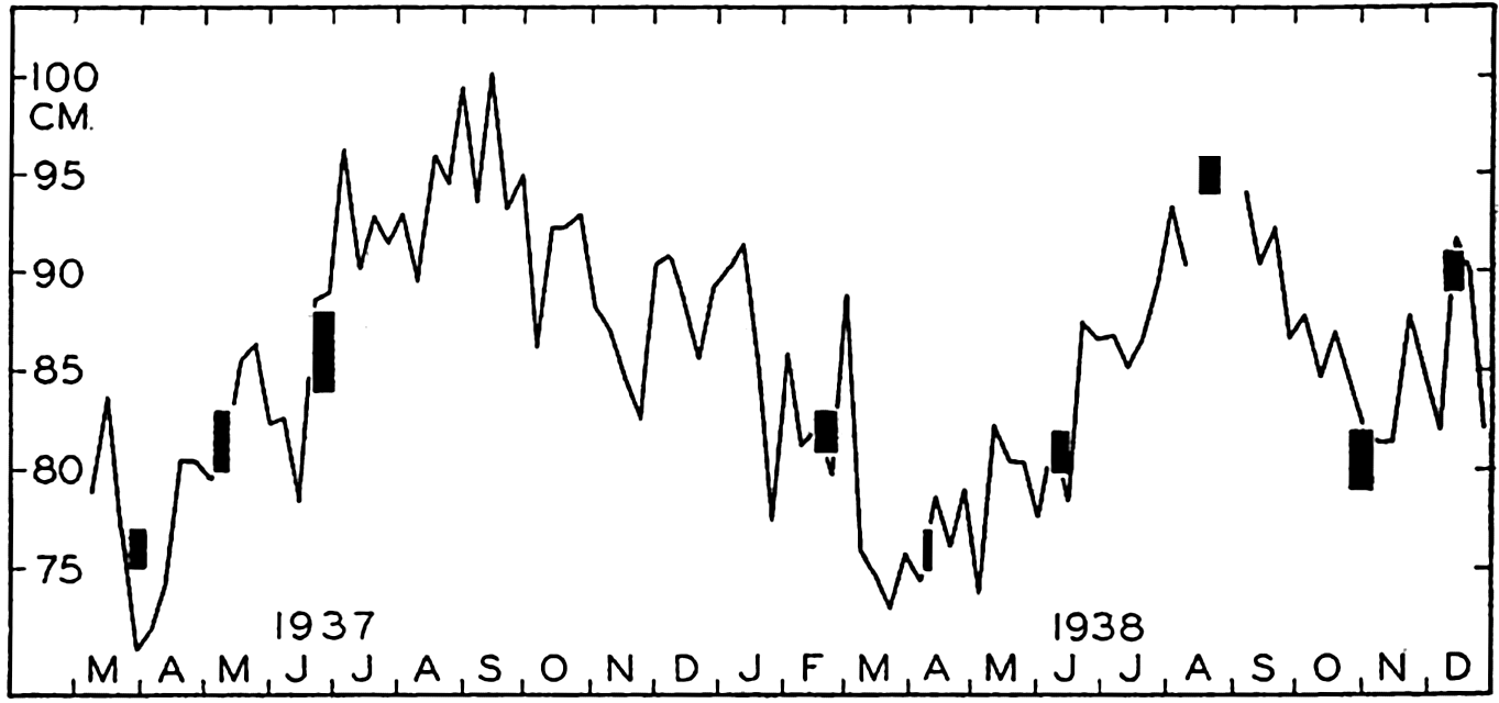
Variations of sea level at La Jolla, California, according to tidal records (curve), and according to observed variations in density above a depth of 500 m (columns).
Sea level on the Pacific coast is about 50 cm higher than on the Atlantic coast, and this difference may perhaps be related to the lower average density of Pacific water.
Variations in the average density of water columns appear capable of accounting for local variations in sea level, as is demonstrated by recent studies of Montgomery (1938) and LaFond (1939). The curve in fig. 111 (LaFond, 1939) shows weekly averages of sea level according to tidal records at La Jolla, California, and the black columns represent the sea level at La Jolla as extrapolated from charts showing the topography of the surface relative to the 500-decibar surface as derived from cruises in 1937 and 1938. The 500-decibar surface was used as reference because near the coast water of uniform density was encountered below a depth of 500 m. Columns have been entered instead of dots because extrapolation of the contour lines as far as the coast is uncertain. The height of the columns gives the probable limits within which sea level on the coast should lie, and the width corresponds to the length in time of the cruises. The agreement between the variations of sea level as
Off a coast near which the density of the coastal water may vary owing to external influences (whereas the density of the oceanic water remains relatively constant), the variations in sea level have direct bearing on the slope of the sea surface toward or away from the coast. Variation in sea level can thus be interpreted in terms of slope of sea surface—that is, in terms of a coastal current. Similarly, if a current flows between an island and a coast, there must be a difference in sea level across the current. Simultaneous registrations of sea level on the island and on the coast may be very helpful in detecting changes of the slope and, thus, in changes in the velocity of the current. For the purpose of detecting such changes, the Woods Hole Oceanographic Institution, with the cooperation of the U. S. Coast and Geodetic Survey, has established a permanent tidal station on Cat Cay, one of the Bimini Islands, which lies on the southeastern side of the Strait of Florida. The records at this station will be compared to those at Key West and Miami, Florida. It can be expected that these studies, which deal with variations in the slope, will amplify the knowledge of the total field of pressure.
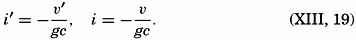
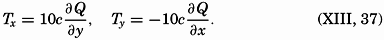
Bjerknes' Theorem of Circulation. The general formula for computing ocean currents from the slope of the isobaric surfaces, ν =−gci, was derived by H. Mohn in 1885, but Mohn did not discriminate sharply between the slope due to internal distribution of mass and the slope due to external factors. Furthermore, the oceanographic observations at the time when Mohn presented his theory were not sufficiently accurate for computation of the relative field of pressure. Owing to these circumstances, and also to others depending on certain characteristics of the theory that have recently been explained by Ekman (1939), Mohn's formula received no attention. The corresponding formula for computation of currents associated with the relative distribution of pressure,
Bjerknes makes use of the term “circulation along a closed curve.” Consider a closed curve that is formed by moving particles of a fluid. The velocity of each particle has a component νs along the curve, and
 .
.If friction is neglected, the time change of the circulation can easily be found from the equations of motion, because
Consider, first, conditions in a coordinate system that is at rest and assume that gravity is the only external force. The integral of the component of gravity along a closed curve is always zero, because it represents the work performed against gravity in moving a particle along a certain path back to the starting point. There remains, therefore, only

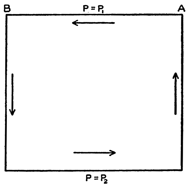
Location in the pressure field of a curve along which the time change of circulation is examined.
If the circulation relative to the earth is considered, the deflecting force has to be taken into account. According to Bjerknes, this is done by writing
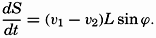
Consider the same curve as before, and assume that the upper line, p = p1, moves at a velocity ν1 at right angles to the line A−B, whereas the lower line, p = p2, moves at a velocity ν2, and let the distance A−B be called L. Then the time change of the projection on the equator plane is
Assume now that the circulation is constant (dC/dt = 0). It then follows that the velocity difference, ν1 − ν2, must be expressed by the equation
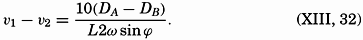
*In the literature, some confusion exists as to the signs in these equations. The above signs are consistent with the coordinates used. The relative velocity is positive; that is, the relative current is directed away from the reader if A lies to the right of B and if DA is greater than DB.
The complete theorem of circulation contains a great deal more than the simple statement expressed by equation (XIII, 32), but so far it has not been possible to make more use in oceanography of Bjerknes' elegant formulation of one of the fundamental laws governing the motion of nonhomogeneous fluids.
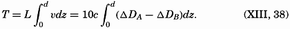
Transport by Currents. The volume transport by horizontal currents has the components
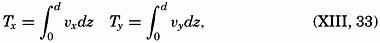
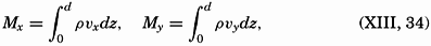
The absolute volume transport can be computed only if the absolute velocities are known, but the volume transport by relative currents can be derived from the distribution of mass. By means of equations (XIII, 16), one obtains

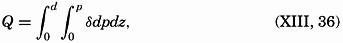
The quantity Q is easily computed, because ΔD is always determined if velocities are to be represented.
It should be observed that in practice the numbers that represent the geometric depths are also considered as representing the pressures in decibars (p. 410). In computing Q the integration is therefore carried to the pressure p decibars and the depth d meters, which are both expressed by the same number, but a small systematic error is thereby introduced. Jakhelln (1936) has examined this error and has shown that the customary procedure leads to Q values that are systematically 1 per cent too small, but this error is negligible.
Curves of equal values of Q can be drawn on a chart, and these curves will bear the same relation to the relative volume transport that the curves of ΔD bear to the relative velocity, provided that the derivations of Q are taken as positive in the direction of decrease. Therefore, the direction of the volume transport above the depth to which the Q values are referred will be parallel to the Q lines, and numerical values will be proportional to the gradient of the Q lines. The factor of proportionality will depend upon the latitude, however; between two Q lines that indicate transport to the north, the transport will increase in the direction of flow, whereas, between two Q lines indicating transport to the south, the transport will decrease in the direction of flow. Taking this fact into account, one can construct curves between which the transport is constant, but these curves will no longer be exactly parallel to the direction of the transport. Within a small area the deviation will be imperceptible, but within a larger area it will be considerable.
Between two stations A and B (A lying to the right), at distance L, the volume transport is
It is not necessary to develop corresponding equations for the mass transport, because this can be derived with sufficient accuracy from the volume transport by multiplication with an average density (Ekman, 1929, 1939; Jakhelln, 1936).
Convenient formulae for the computation of the transport of a coastal current have been developed by Werenskiold (1937) on the assumption that the isosteres rise toward the surface and intersect the surface at some distance from the coast (see fig. 113).
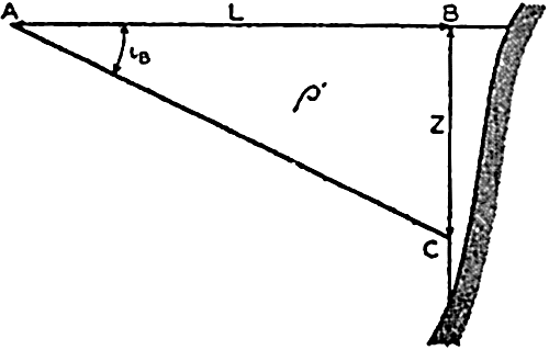
Schematic representation of hydrographic conditions off a coast.
If there are only two layers of homogeneous water, the transport is easily found. If the water of greatest density is at rest, the velocity in the area ABC (fig. 113) is
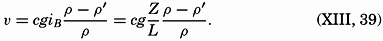
The volume transport apparently has been computed from observations at only the one station at which the depth to the boundary surface is Z, but the assumption that at and beyond the distance L the homogeneous, denser water reaches surfaces is equivalent to assuming that conditions at a second station at or beyond L are known. Owing to this circumstance, it is readily seen that the boundary surface can have any shape, because it has already been shown that the transport between two stations depends only upon the distribution of density at the two stations and is independent of the distribution of density between the stations.
For currents in water within which the density varies continually with depth, Werenskiold arrives at the formula
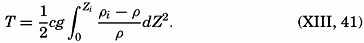
A consideration of computed transport and of the continuity of the system is helpful, under certain conditions, in separating currents flowing one above the other. The average transport through a vertical section that represents the opening to a basin must be zero, because water cannot accumulate in the basin, nor can it continue to flow out of the basin. Observations at stations at the two sides of such a section may, however, show transport in or out if the velocity along the bottom is assumed to be zero. However, this assumption would be wrong, and a depth of no motion must be determined in such a manner that the transport above and below that depth are equal. This depth can be found by plotting the difference ΔDA − ΔDB against depth, computing the average value of the difference between the surface and the bottom, and reading from the curve the depth at which that average value is found. This depth is then the average depth of no motion, and the transports above and below that depth are in opposite directions.
Determination of the depth above and below which the transport between two stations, A and B, is equal.
The procedure is illustrated in fig. 114, in which is plotted the difference ΔDA − ΔDB at Meteor stations 46 off South America and 23 off South Africa, both in about latitude 29°S. Assuming no current at a depth of 3500 m, one would obtain a transport to the north proportional to the area ABC, or equal to 44.5 million m3/sec. Such a transport to the north is impossible, and the velocity must therefore be zero at some other depth. The average value of ΔDA − ΔDB is 0.090 dynamic meters, and this value is found at a depth of 1325 m. If this depth is selected as a depth of no motion, the transport to the north becomes proportional to the area DBE and equal to 20.7 million m3/sec, and below 1325 m the transport is directed to the south, is proportional to the area ECF, and is also equal to 20.7 million m3/sec. The transport above the depth of no motion can be written in the form

Only the average depth of no motion can be determined in this manner. Generally, the depth of no motion is not constant, but the inclination can be found by studying the distribution of temperature and salinity in the section. It is rational to assume that a surface of no motion coincides with isothermal and isohaline surfaces, and that therefore, in a section, the depth of no motion follows the isotherms and isohalines. On that assumption, one finds that in the example which has been discussed the depth of no motion rises from about 1450 m off South America to about 1200 m off South Africa.
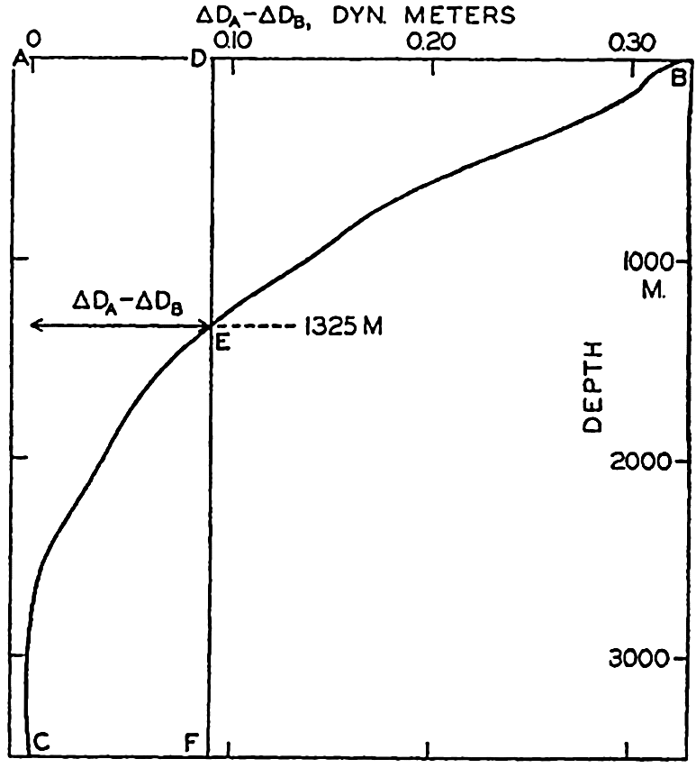
Deflections of a current when passing a ridge, the profile of which is shown at the bottom. Left. Deflection of a current in homogeneous water, due to friction (Ekman). Right. Deflection of a relative current (see fig. 116).
The Influence of Bottom Topography on Ocean Currents. Ekman (1923, 1927, 1932) has examined the effect of the bottom topography on currents, taking into account the rotation of the earth. He arrived at the conclusion that in low latitudes the currents tend to flow east-west, independent of the slope of the bottom, but that in middle and high latitudes the currents tend to follow the bottom contours. These conclusions are verified by experience. Ekman also found that a current will be deflected cum sole when entering shallower water and contra solem when entering deeper water, and that these deflections are independent of the absolute depth to the bottom. The curvature of the stream lines is greatest where the change in slope is greatest, and when crossing a ridge the stream lines will therefore have the form shown in fig. 115, left.
In his examination, Ekman assumed homogeneous water and the presence of a slope current within which the velocities are independent of depth except within a layer that is influenced by bottom friction (p. 499). The effect of the bottom topography on relative currents in non-homogeneous water has not been examined, but qualitatively the character of the modifications is easily seen. Consider first, in the Northern Hemisphere, a relative current which in an ocean of constant depth reaches nearly to the bottom (fig. 116). Within such a current the deepest isopycnic or isosteric surfaces are horizontal, but above the
 (δ1 − δ2) expresses the relation between the slope of the isobaric surface, ip, and the average slope of the δ surfaces,
  (p. 412). This distribution of mass and pressure is illustrated on the right-hand side of the perspective diagram in fig. 116, where it is supposed that the isosteric surface δ = δ1 coincides with a level surface.
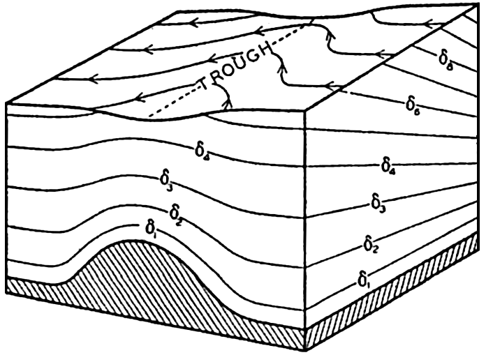
Perspective diagram showing the deformation of the sea surface when a relative current reaching nearly to the bottom crosses a submarine ridge.
When this current approaches a submarine ridge over which the water must flow, the δ surfaces must rise, as shown in the diagram. Accordingly, the distribution of mass is altered in the direction of flow in such a manner that the δ surfaces slope upward when approaching the ridge and downward after passing the ridge. The isobaric surfaces are altered correspondingly and must slope downward when the current approaches the ridge and upward after it has passed; that is, a low-pressure trough develops along the ridge, but this trough rises from left to right relative to an observer who looks in the direction of flow, because the lighter water remains on the right-hand side (fig. 116). Consequently, the isohypses of the isobaric surfaces, which were straight lines over the even bottom, bend to the right when the current approaches the ridge and to the left when it has passed. In the Southern Hemisphere the bends will be in opposite directions, and, in general, a deep current is therefore deflected from its straight course when crossing a ridge, the deflection being to the right in the Northern Hemisphere and to the left in the Southern. The maximum deflection in this case is directly over the ridge, as shown in fig. 115.
In the schematic representation in fig. 116 the δ surfaces at intermediate depths—say, the surfaces marked δ3 and δ4—must evidently show a ridge above the bottom ridge and must at the same time slope from left to right. The σt surfaces must have a similar form. As an example of such influence of the bottom topography on the field of mass, fig. 117 shows the topography of the surface σt = 27.7 in the region where
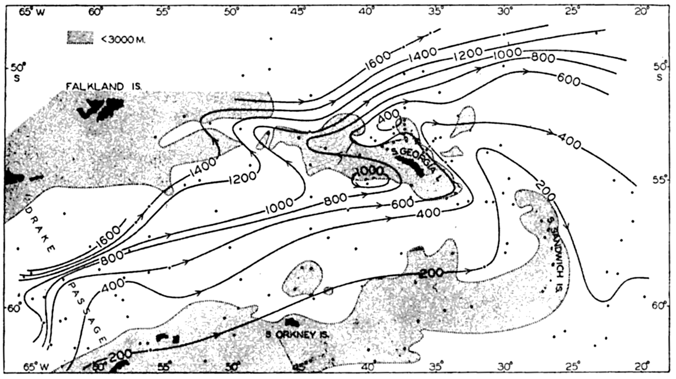
Topography of the surface σt = 27.7 in the area from the Drake Passage to the east of South Sandwich Islands.
Qualitative examples other than the one shown in fig. 116 can easily be prepared. Thus, the current must flow around a peak rising from the sea bottom, and this flow will result in a widening of the distance between the stream lines above the peak and perhaps in the development of a cyclonic eddy. The discussions by Wüst (1940) and Neumann (1940) of conditions around the Altair dome in the North Atlantic confirm these conclusions.
The above reasoning is purely qualitative. If the quantitative effect of the bottom topography is to be examined, it is necessary to consider that the equation of continuity and the equations of stationary motion and stationary distribution of mass must be satisfied. No quantitative computations have been made, but it can be pointed out that stationary distribution of mass requires that the law of the parallel solenoids be fulfilled (p. 455). Hence the isohypses of all isobaric
Friction
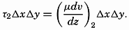
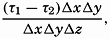
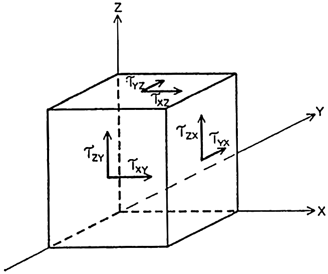
General Consideration of Friction. Two of the fundamental concepts concerning friction in a fluid are (1) that shearing stresses are produced when layers are slipping relative to each other, and (2) that the shearing stresses acting on a unit area are proportional to the rate of shear normal to the surface on which the stress is exerted: τ = μdv/dn. The factor of proportionality, μ, is called the dynamic viscosity of the fluid.
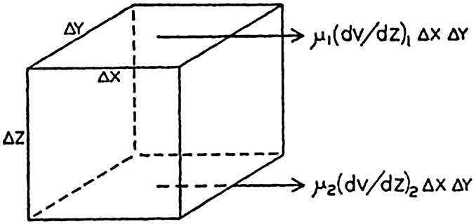
Frictional stresses in the direction of the x axix on two sides of a cube.
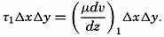
Frictional forces per unit volume are equal to the differences between shearing stresses exerted on opposite sides of a cube of unit dimensions. Consider a cube of side length Δz (fig. 118) in a fluid moving only in the direction of the x axis, and let the rate of shear at the upper and lower surfaces of the cube be (dv/dz)1 and (dv/dz)2, respectively. The shearing stress per unit area of the upper surface is then τ1 = (μdv/dz)1, and the total stress acting on the upper surface is
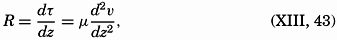
In classical hydrodynamics the dynamic viscosity, μ, is considered a characteristic property of the fluid—namely, the property that resists angular deformation. Being a characteristic property, the magnitude of μ is independent of the state of motion, but it varies, as a rule, with the temperature of the fluid. Within wide limits it is independent of the pressure. The dynamic viscosity has the dimensions ML−1T−1, whereas the kinematic viscosity, defined as ν = μ/ρ, has the dimensions L2T−1. A table of the dynamic viscosity of sea water is given on p. 69.
The derivation of the general frictional terms that must be taken into account when dealing with motion in space is given in the general textbooks on hydrodynamics or fluid mechanics which are listed at the end of this chapter. The complete theory requires the introduction of both shearing and normal stresses, and leads, if μ is considered constant, to the expressions for the frictional terms:
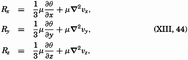
 .
.When these terms are added to the equations of motion (XIII, 1), and if the terms depending upon the divergence of the velocity are omitted, one obtains the Navier-Stokes equation of motion (for example, Lamb, 1932), which in greatly simplified form has found application to problems in fluid mechanics. The theory that leads to the development of the Navier-Stokes equation excludes, however, the possibility of local fluctuations in velocity and presupposes that the fluid moves in layers, or laminae. This type of motion is called “laminar flow,” but is probably never encountered in the ocean. The Navier-Stokes equations find, therefore, no application to oceanographic problems and have been mentioned here only as an approach to the problem of fluid resistance
Turbulence. Laminar flow, in which sheets of fluid move in an orderly manner is, as has already been stated, not known to occur in the ocean. The ocean currents are, instead, characterized by numerous eddies of different dimensions by which small fluid masses are constantly carried into regions of different velocity. It is this completely irregular type of motion which is called turbulent flow, and the process by which a rapid exchange of fluid masses is maintained is called turbulence.
The very character of turbulent flow is such that rapid fluctuations of velocity take place in all localities, and no steady state of motion exists if attention is paid to the individual particles of the fluid. It might therefore appear hopeless to arrive at a theory that takes full account of the complicated character of the actual motion, but the problem has, nevertheless, been attacked with considerable success by using statistical methods. The velocity at any given point in space can always be considered as the vector sum of two different velocities:  , which represents the average velocity at that point during a long period of time, and ν′ which represents the added “turbulent” velocity. At any given time the actual velocity components can therefore be written

After such a segregation is made, the whole pattern of flow can be considered as composed of two systems, one representing the average flow, which may be steady or accelerated, according to the acting forces, and one representing the irregular turbulent motion, which is superimposed upon the average flow and whose nature is not known at any given time. The former system, the average flow, is of interest when dealing with the ocean currents, but knowledge of the superimposed turbulent flow is necessary for studying the extent to which the turbulent flow modifies the apparent viscosity.
Frictional Stresses Due to Turbulent Motion. It is not possible here to present the complete development of the frictional terms. Interested readers are referred to general textbooks on hydrodynamics or fluid mechanics (for example, Lamb, 1932, Rouse, 1938), but a few important points must be brought out here. Owing to the very character of the turbulent motion, small fluid masses are carried back and forth across any given surface, and a mass coming from a region of high velocity has, when entering a region of low velocity, a momentum which is greater than that of the surrounding particles. If this fluid mass assumes approximately the velocity of the surroundings, it loses momentum, and, similarly, a small fluid mass that comes from a region of low velocity into one of high velocity gains momentum. Thus, where a
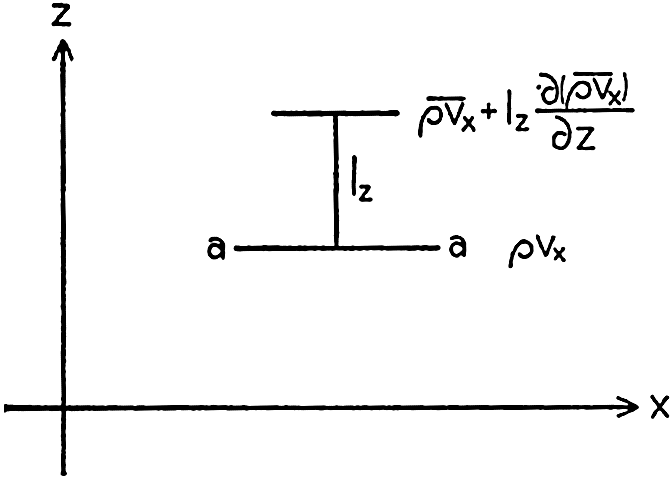
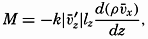
Change of momentum on the vertical distance lz.
Reynolds first derived expressions for the stresses due to momentum transport, and since then the theory of turbulence has been further developed, notably by L. Prandtl, G. I. Taylor, and Th. v. Kármán. The method of attack which so far has found the greatest application to oceanographic problems is based on Prandtl's introduction of the mixing length. Consider that the average flow is in the direction of the x axis and that  . Then
 between the average original momentum of the small fluid masses
  and the average momentum at the locality where exchange takes place. The momentum given off per unit time must be proportional to the average numerical value of the vertical velocity of the small fluid masses, which is
  . Therefore, the rate of momentum transport, M, will be

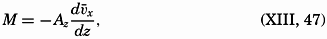
Prandtl's theory also leads to another definition of Az:
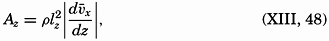
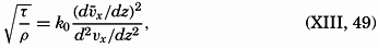
The above considerations lead to the result that
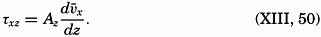
Equation (XIII, 50) is similar to the equation τ = μdv/dn (p. 69). The coefficient Az has the same dimensions as the dynamic viscosity μ and is called the eddy viscosity. However, a fundamental difference exists between the two quantities. The dynamic viscosity is independent of the state of motion and is a characteristic property of the fluid, comparable to the elasticity of a solid body, but the eddy viscosity depends upon the state of motion and is not a characteristic physical property of the fluid. The numerical value of the eddy viscosity varies within very wide limits according to the type of motion, and, as far as ocean currents are concerned, only the order of magnitude of Az has been ascertained.
It should be observed that the eddy viscosity can be introduced without paying any attention to the mixing length or any other statistical quantity that describes the character of the turbulence. Because in a
 , where
  stands for the mean motion and where A evidently must depend upon the character of the turbulence. This notation was used by Ekman (1905) in his classical discussion of wind currents, in which the eddy viscosity was first introduced analytically under the name “virtual viscosity” when dealing with oceanographic problems.
For the sake of completeness, it may be added that the expression for the stress should also contain the term  , but this can always be neglected, because μ is very small compared to A. Oceanographic data give values of A ranging between 1 and 1000 g/cm/sec, whereas μ is about 0.015 (table 16, p. 69).
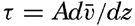
Shearing stresses acting on three sides of a cube.
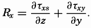
The discussion of the shearing stresses due to turbulent exchange of momentum can now be extended by dropping the assumption that the motion takes place in the direction of the x axis only, because the reasoning is equally correct if the average velocity has a component in the direction of the y axis. The stress in the direction of the y axis on a surface normal to the z axis, τyz, is
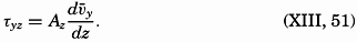
Dropping the assumption that  = 0 and that the average velocity does not vary in a horizontal direction leads to the introduction of four new shearing stresses (fig. 120):
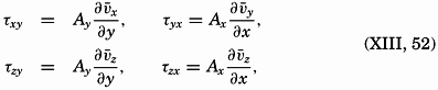
Here the coefficients of eddy viscosity may be defined as before:

Frictional Forces Due to Turbulent Motion. The frictional force acting in the direction of the x axis is derived from the stresses τxz and τxy (fig. 120):
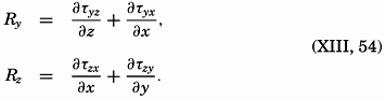
In order to arrive at frictional terms that are of importance when dealing with ocean currents, it will be assumed that (1) only the shearing stresses that have been discussed here are important, (2) the vertical velocity is so small that the gradients of the vertical velocity are negligible, and (3) the horizontal mixing length and the average horizontal turbulent velocities are independent of the direction of motion; that is, Ax = Ay = Ah. Writing simply νx instead of  , and so on, one obtains the frictional terms in the form
The above derivation is not an exact one, and therefore the equations that define the frictional forces in the ocean represent only approximations that appear satisfactory at the present stage of knowledge of ocean currents. When it becomes desirable to improve these expressions, it will be necessary to consult the treatment of the problem of fluid friction which is given in the textbooks on hydrodynamics or fluid mechanics listed at the end of this chapter.
In applying the expressions for the frictional forces, a further simplification is generally be introduced—namely, that the horizontal frictional forces can be disregarded. The concept of horizontal turbulence, however, has been introduced because horizontal or quasihorizontal turbulence appears to play an important part in large-scale processes of diffusion, although the dynamic significance is not yet clear.
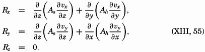
If horizontal turbulence is neglected, the consideration of transport of momentum leads to the frictional terms
Influence of Stability on Turbulence. No theory has been developed for the state of turbulence which at indifferent equilibrium or at stable stratification characterizes a given pattern of flow, except in the immediate vicinity of a solid boundary surface (p. 480), but it has been demonstrated that the turbulence as expressed by the eddy viscosity decreases with increasing stability. Thus, Fjeldstad (1936) found that he could obtain satisfactory agreement between observed and computed tidal currents in shallow water by assuming that the eddy viscosity was a function not only of the distance from the bottom but of the stability as well. He introduced A = f(z)/(1 + aE), where E is the stability and where the factor a is determined empirically.
The relation between eddy viscosity and eddy diffusion has been examined by Taylor (1931). Taylor's reasoning is based on the fact that, in the presence of turbulence, the kinetic energy of the system can be considered as composed of two parts: the kinetic energy of the mean motion, and the kinetic energy of the superimposed turbulent motion. In homogeneous water the latter is being dissipated by viscosity only, wherefore, if the turbulence remains constant, turbulent energy must enter a unit volume at the same rate at which it is dissipated. Where stable stratification is found (p. 92), part of the turbulent energy is also used for increasing the gravitational potential energy of the system. In this case the rate at which turbulent energy enters a unit volume, T, must equal the sum of the rate at which the potential energy increases, P, and the rate at which energy is dissipated by viscosity, D. It follows that, if the turbulence remains unaltered, one must have T > P.
Taylor shows that the rate at which turbulent energy enters a unit volume equals  , where Av means the eddy viscosity, and that the rate at which the potential energy increases equals gEAs, where E is the stability (p. 416) and As is the eddy diffusivity. It follows that
Taylor tested the correctness of this conclusion by measurements made by Jacobsen (1913) in Danish waters, where Jacobsen found values
According to Taylor's theory, turbulence can always be present, regardless of how great the stability is, but the type of turbulence must be such that the condition (XIII, 57) is fulfilled; that is, the rate at which the Reynolds stresses communicate energy to a region must be greater than the rate at which the potential energy of that region increases. It explains why observations in the ocean mostly give smaller values of As than of Av. A velocity gradient of 0.1 m/sec on 100 m is common where the stability is about 10−6 m−1, and with these values one obtains As < 0.1Av. Within layers of very great stability the velocity gradient is generally also great, but the value of As becomes even smaller than in the above example. Thus, below the Equatorial Countercurrent in the Atlantic the decrease of velocity in a vertical direction is 6.10−3 sec−1, and the stability is about 5.10−5 m−1 (Montgomery, 1939). With these values, one obtains As < 7.10−2 Av, or, if the eddy viscosity were equal to 10 g/cm/sec, the eddy diffusivity would be less than 0.7.
Thus the effect of stability on turbulence is twofold. In the first place, the turbulence is reduced, leading to smaller values of the eddy viscosity, and, in the second place, the type of the turbulence is altered in such a manner that the accompanying eddy diffusivity becomes smaller than the eddy viscosity. The latter change is explained by Jacobsen (1930) by assuming that elements in turbulent motion give off their momentum rapidly to their surroundings, but that other properties are exchanged slowly, and that before equalization has taken place the elements are moved to new surroundings by gravitational forces (p. 92). A possible influence of stability on lateral turbulence has not been examined, but it has been suggested by Parr (1936) that this kind of turbulence increases with increasing stability.
Horizontal Turbulence. The horizontal turbulence needs some further explanation because of the effect of the earth's rotation. Let it be assumed that the field of pressure is such that the deflecting force associated with the mean motion is balanced by the pressure gradient:
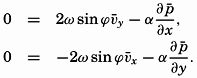
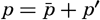 , one finds that the above equations must take the form
 and
and  represent the mean pressure gradients, and −∂p′/∂x and −∂p′/∂y represent local pressure gradients associated with the turbulent motion.
Thus, superimposed upon the average field of pressure must be an irregular field. If the pressure distribution could be represented by means of the absolute geopotential topographies of isobaric surfaces (p. 413), these would show, besides certain major features that would characterize the mean motion, also a number of small “lows” and “highs,” troughs and ridges, which would represent the superimposed irregular pressure field. Detailed surveys during which the oceanographic stations have been spaced at intervals of 20 km or less have revealed that the relative distribution of pressure shows numerous irregularities of such nature. This fact strongly supports the conclusion that the horizontal motion associated with the pressure distribution is far from being uniform, but is characterized by numerous eddies that may have dimensions up to 20 km or more.
Boundary Friction. In oceanography the problem of frictional stresses at boundary surfaces can be dealt with in the same manner as the similar problem in fluid mechanics. Over an absolutely smooth surface
Over a rough surface, different conditions are encountered. Prandtl assumes that over such a surface the turbulent motion extends to the very surface, meaning that the mixing length has a definite value at the surface itself:

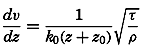
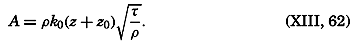
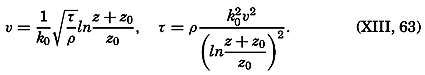
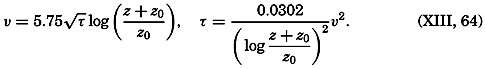
Measurements of the velocity at two distances are needed in order to determine both τ and z0, and measurements at three or more levels are necessary in order to test the validity of the equation. So far, few measurements have been made so close to the bottom that they can be used for testing the application of these results to oceanographic conditions, but one example can be given. On November 15, 1937, Revelle and Fleming (unpublished data) measured tidal currents off the entrance to San Diego Harbor at 126, 51, and 21 cm above the bottom. Table 63 contains the average velocities and the stress at the bottom, if the bottom is assumed to be smooth or rough. Agreement is obtained only if the bottom is considered rough. The roughness length is found to be about 2.0 cm, and with this value the observations consistently give the same stress at the bottom. These observations indicate therefore that the above formulae, with von Kármán's constant, k0 = 0.4, are applicable to the currents directly above the sea bottom. In this case the value of the eddy viscosity would be A = 0.93 (z + z0); that is, at a distance of 1 m above the bottom the eddy viscosity would be 95 g/cm/sec.
| Distance from bottom, cm | 126 | 51 | 21 |
| Average velocity, cm/sec | 26.3 | 21.6 | 15.6 |
| Computed frictional stress, g/cm/sec2} Smooth bottom | 0.87 | 0.71 | 0.46 |
| Computed frictional stress, g/cm/sec2} Rough bottom, z0 = 2.0 cm | 5.8 | 6.2 | 6.0 |
The above results apply to a fluid in a state of indifferent equilibrium. Certain modifications must be introduced if the stratification is stable or unstable, but the character of these modifications is not fully understood. It can be stated only that under stable conditions the velocity profile at some distance from the surface can no longer be represented by a logarithmic law, but is better represented by a power law of the type Vz1/Vz2 = (z1/z2)n. However, very near the surface, the logarithmic law appears to be valid (Sverdrup, 1939b).
At the sea surface, different boundary conditions have to be considered. In the first place, it should be observed that the currents of the sea are always much slower than the air currents, the winds. Therefore the velocity of the air relative to that of the water can always be considered, with sufficient accuracy, equal to the velocity of the wind.
At the sea surface the stress that the wind exerts on the water, τa, must balance the stress that the water exerts on the air:
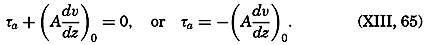
When a current flows parallel to a coast, a lateral stress is exerted, and one may expect a horizontal velocity profile to develop which shows some similarity to the vertical profile near the bottom. The velocity profile must be related to the horizontal eddy viscosity and to the lateral stress, but this relation has not yet been examined.
Numerical Values of the Vertical and Lateral Eddy Viscosity and Eddy Diffusivity. For the determination of the eddy viscosity, Aν., in the ocean, it is necessary to know the frictional forces and the velocity gradients. The frictional forces cannot be determined directly, but may be obtained as the difference between other acting forces. The velocity gradients, however, can be obtained from directly obseryed currents. When dealing with wind currents, theories based on certain assumptions as to the character of the eddy viscosity are helpful (p. 492), and for considering currents close to the bottom, results from fluid mechanics make possible conclusions as to the eddy viscosity from current measurements only (p. 480). The uncertainties of the correct application of theories, the difficulties in making current measurements in the open ocean, and the even greater difficulties in determining the acting forces, all introduce great uncertainties in the numerical values of the eddy viscosity which have so far been determined.
Table 64 contains results of such determinations. The specific methods used cannot be discussed here, but some of them will be mentioned later on. All values are from regions of moderate or strong currents that have been measured with considerable accuracy, or they have been derived from the effect of wind currents on the surface layer. The values range from nearly zero up to 7500 g/cm/sec, but some consistency in the variations can be seen. At the very bottom, small values are always found; at greater distances from the bottom, great values are associated with strong currents and small stability or with strong currents and great stability. On the North Siberian Shelf the eddy viscosity approached a small value in a thin layer of very great stability within which the tidal currents reached their maximum values.
| Locality | Layer | Av in g/cm/sec | Av derived from | Authority |
aW = wind velocity in m/sec. | ||||
bz = distance from bottom in meters. | ||||
cVery great stability. | ||||
dVery strong currents. | ||||
ez = distance from bottom in meters. Formula valid between z = 0.2 and z = 1.3 m. | ||||
| All oceans | surface | [a]Av = 1.02 W3 (W<6m/sec) | homogeneous layer | Thorade, 1914 |
| Av = 4.3 W2 (W >6m/sec) | Thickness of upper | Ekman, 1905 | ||
| North Siberian Shelf | 0 to 60 m | 0−1000 | Tideal currents | Sverdrup, 1926 |
| North Siberian Shelf | 0 to 60 m | 10−400 | Tidal currents | Fjeldstad, 1936 |
| North Siberian Shelf | 0 to 22 m | [b] | Wind currents | Fjeldstad, 1929 |
| North Sea | 0 to 31 m | 75−1720 | Strong tidal currents | Thorade, 1928 |
| Danish waters | 0 to 15 m | [c] 1.9−3.8 | All currents | Jacobsen, 1913 |
| Kuroshio | 0 to 200 m | [d] 680−7500 | All currents | Suda, 1936 |
| Japan Sea | 0 to 200 m | 150−1460 | All currents | Suda, 1936 |
| Off San Diego, Calif | near bottom | [e] 93(z + 0.02) | Tidal currents | Revelle and Fleming, ms. |
By computations that are based on equation (V, 5), p. 159, in a simplified form, the eddy diffusivity, As can be derived from observed time and space variations of temperature, salinity, oxygen content, or other properties. In some cases the currents need not be known, but in other cases only the ratio As/v can be determined, where ν is the velocity of the currents (p. 159). If this velocity can be estimated, an approximate value of As can be found. Temperature, salinity, and oxygen content can be measured much more easily and with greater accuracy than currents, and data for studying the eddy diffusion are therefore more readily obtained. As a consequence, many more determinations of eddy diffusivity have been made, and the results show greater consistency.
Table 65 contains a summary of values derived from observations in different oceans and at different depths between the surface and the bottom. The values range from 0.02 up to 320 g/cm/sec, but by far the greater number of values lie between 3 and 90. The range is therefore smaller than the apparent range of the eddy viscosity. The highest value, 320 g/cm/sec, was found in a homogeneous surface layer, within which one can expect the eddy diffusivity to equal the eddy viscosity. This value is the only one which is as great, probably, as the corresponding eddy viscosity; otherwise, the eddy diffusivity is smaller, in agreement with the fact that generally stable stratification is encountered. From the remarks in the table, it is evident that the eddy diffusivity increases with increasing velocity of the currents and decreases with increasing stability, in agreement with the preceding considerations.
The results of a few determinations of lateral eddy coefficients are given in table 66. The values of the coefficients have been derived by bold assumptions and can be considered as indicating only the order of magnitude. The fact that this order of magnitude depends upon the size of the area from which observations are available probably explains why the value from the California Current is much smaller than the values from the Atlantic Ocean, where conditions within much larger regions have been considered. The latter values, which have been obtained partly from observations at or near the surface and partly from observations at great depth, agree remarkably well. No relation appears between the average velocity of the currents and the eddy coefficients or between the stability and the coefficients. Similarly, from the meager evidence, the eddy viscosity and eddy diffusivity appear to be equal. Therefore, the processes of lateral turbulence seem to be entirely different from those of vertical turbulence, but it should be borne in mind that the study of lateral turbulence in the ocean is at its very beginning.
| Locality | Layer | As in g/cm/sec | Remarks | Authority |
| Equatorial Atlantic Ocean | 0 to 50 m | 320 | Homogeneous water, moderate currents | Defant, 1932 |
| Bay of Biscay | 0 to 100 m | 2–16 | Moderate stability, weak currents | Fjeldstad, 1933 |
| Danish waters | 0 to 15 m | 0.02–0.6 | Great stability, moderate currents | Jacobsen, 1913 |
| Kuroshio | 0 to 200 m | 30–80 | Moderate stability, strong currents | Sverdrup et al, 1942 |
| Kuroshio | 0 to 400 m | 7–90 | Moderate stability, strong currents | Suda, 1936 |
| Japan Sea | 0 to 200 m | 1–17 | Moderate to small stability, moderate currents | Suda, 1936 |
| California Current | 0 to 200 m | 30–40 | Moderate stability, weak currents | McEwen, 1919 |
| Arctic Ocean | 200 to 400 m | 20–50 | Small stability, weak currents | Sverdrup, 1933 |
| South Atlantic Ocean | 400 to 1400 m | 5–10 | Moderate stability, weak currents | Defant, 1936 |
| Equatorial Atlantic Ocean | 600 to 2000 m | 8 | Moderate stability, weak currents | Seiwell, 1935 |
| Caribbean Sea | 500 to 700 m | 2.8 | Moderate stability, weak currents | Seiwell, 1938 |
| South Atlantic Ocean | 3000 m to bottom | 4 | Homogeneous water, weak currents | Defant, 1936 |
| South Atlantic Ocean | Near bottom | 4 | Homogeneous water, weak currents | Wattenberg, 1935 |
| Locality | Layer | Av,h or As,h in g/cm/sec | Remarks | Authority |
| Northwestern North Atlantic Ocean | Surface | As,h 4 × 10⁸ | Strong currents | Neumann, 1940 |
| Atlantic Equatorial Countercurrent | 0 to 200 m | Av,h 7 × 10⁷ | Great stability, moderate currents | Montgomery and Palmén, 1940 |
| 0 to 200 m | As,h 4 × 10⁷ | Montgomery, 1939 | ||
| South Atlantic Ocean | 2500 to 4000 m | As,h 1 × 10⁸ | Small stability, weak currents | Sverdrup, 1939a |
| California Current | 200 to 400 m | As,h 2 × 10⁶ | Moderate stability, weak currents, small area | Severdrup and Fleming, 1941 |
The Energy Equation When Friction Is Taken into Consideration. Because explicit terms for the components of the frictional forces have been introduced, the total power of the frictional forces can be computed. Disregarding the effect of horizontal turbulence, the power of the frictional forces per unit volume is
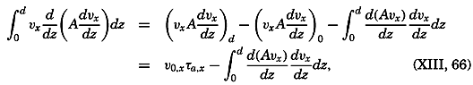
The integral on the right-hand side represents the loss per unit time and unit surface area of kinetic energy due to the vertical turbulence (the dissipation). If A were constant, the integral would be reduced to
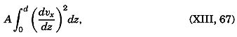
The first term on the right-hand side, ν0,τa, represents the power per unit area (ML2T−3 × L−2) which is exerted by the stress of the wind.
The energy equation can now be written in the form
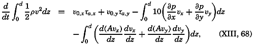
Some general conclusions can be drawn from this equation. In the first place, it is seen that the change of the kinetic energy may be positive or negative; that is, the energy transmitted to the water from the atmosphere may be greater or smaller than the loss due to motion across isobars and dissipation. Furthermore, if the kinetic energy remains unaltered and the stress of the wind is zero, energy must be gained by motion across the isobars; that is, the average motion must be from high to low pressure, because the dissipation is always positive. On the other hand, if the first integral vanishes, the dissipation equals the power of the stress of the wind. The first integral can disappear, either because the term (∂p/∂x)vx + (∂p/∂y)vy is zero at all depths, or because the term is negative at some depths and positive at others. In the former case the motion is parallel to the isobars. Furthermore, if stationary conditions are assumed, the isobars at one level must be parallel to the isobars at another level (p. 455). If the horizontal x axis is placed in the direction of the pressure gradient, the equations of motion are reduced to
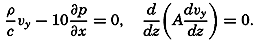
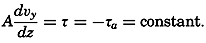

The energy equations have so far received but little attention in oceanographic work, and further theoretical considerations and applications to specific problems appear desirable.
Other conclusions as to the effect of the stress of the wind can be based directly upon an integration of the equations of motion. Consider a closed space in which stationary conditions exist, and assume that the motion is nowhere accelerated. In such a system the transport through any cross section must be zero. Therefore, if the positive x axis is placed in the direction of the wind, one obtains, by multiplying the equations of motion by dxdydz and integrating over the entire volume,
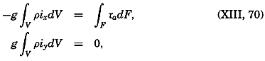

The formula is valid only if the depth to the bottom is so great that the velocity gradient at the bottom is zero, because only on this assumption does the stress at the bottom vanish. If this condition is not fulfilled, one obtains

In nonhomogeneous water, one can write

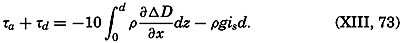
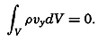
All of the above equations become modified if horizontal stresses and frictional forces related to such stresses are considered, but so far these modifications have not been examined. Rossby (1936a), however, has pointed out that the stress of the wind exerts an anticyclonic torque on the surface of the different oceans and that lateral stresses must provide the balancing cyclonic torque, because the bottom stresses are probably negligible. Studies by Montgomery and Palmén (1940) support this conclusion, but the problem deserves further attention.
Wind Currents
The Stress of the Wind. From laboratory results dealing with flow over smooth and rough surfaces, one may expect that the stress can be expressed by means of equation (XIII, 59), which gives the stress over a smooth surface, or equation (XIII, 63), which gives the stress over a rough surface. The density, ρ, which enters in the formulae is then the density of the air. In order to determine whether the sea surface can be considered smooth or rough and, if it is rough, to determine the value of the roughness length, zo, simultaneous measurements of wind velocities must be made at three or more levels above the sea surface. From such measurements conducted by Wüst (1920), Rossby and Montgomery (1935) concluded that at moderate wind velocities the sea surface has the character of a rough surface with roughness length 0.6 cm. From a general theory of the wind profile in the lower part of the atmosphere, Rossby (1936b) later developed formulae that permit computation of zo from the angle between the surface wind and the gradient wind (corresponding to no friction) or from the ratio between surface-wind velocity and gradient-wind velocity. When applying these formulae to observed values from the ocean, Rossby found that at moderate and strong winds the roughness length is independent of the wind velocity and equal to

A similar expression was derived by Ekman as early as 1905 through study of the slope of the sea surface during a storm in the Baltic in 1872. A. Colding had found that the lines of equal water level were directed nearly perpendicular to the direction of the wind. The sea-level values were obtained from records at stations on the coast, and thus represent the values of the physical sea level. The relation between wind velocity, W, depth, d, and slope, i, could be expressed by the equation
In the case examined by Colding, Ekman assumes that τa + τd = 3/2τa, and obtains, therefore,
Palmén and Laurila (1938) have made a similar study of the effect of the wind on the sea level in the Gulf of Bothnia during a storm in October, 1936, and obtained
These results, although uncertain, confirm the conclusion that at moderate and strong winds the stress of the wind is proportional to
At low wind velocities, somewhat different conditions appear to prevail. From a study of simultaneous wind measurements at different heights above the sea, Rossby (1936b) concludes that at low wind velocities the sea surface has the character of a smooth surface, because the wind profiles indicate the existence of a laminar sublayer. At low wind velocities the stress should therefore be computed from equation (XIII, 59), which gives values that are about one third of those obtained on the assumption that the surface is rough.
Table 67 shows the values of the stress corresponding to a smooth surface or a rough surface characterized by z0 = 0.6 cm.
| Surface | Wind velocity in m/sec at 15 m | ||||||||
|---|---|---|---|---|---|---|---|---|---|
| 2 | 4 | 6 | 8 | 10 | 12 | 14 | 16 | 18 | |
| “Smooth” | 0.04 | 0.16 | 0.34 | (0.58) | |||||
| “Rough” | (0.11) | (0.45) | (1.01) | 1.81 | 2.83 | 4.09 | 5.56 | 7.25 | 9.20 |
It is evident that, if the sea surface can be considered smooth at wind velocities below 6 to 7 m/sec, the stress of wind velocities below this limit is of little significance, but the above conclusions need to be confirmed by means of many more data. The problem of the stress of the wind still deserves great attention, and it is particularly desirable to obtain more measurements of wind profiles, because results in fluid mechanics can be successfully applied in the study of such profiles.
The theoretical equations for the relations between stress and wind velocity are valid only if the stability of the air is nearly indifferent. Under stable or unstable conditions the wind profiles will be different, and the relationships between wind velocity and stress will be altered (Sverdrup, 1939b). A study of wind profiles at different stabilities of the air is therefore of great interest.
Wind Currents in Homogeneous Water. In 1902, V. Walfrid Ekman published his classical paper on wind currents in which, for the first time, the effect both of the deflecting force of the earth's rotation and of the eddy viscosity was taken into account. Ekman undertook the mathematical analysis at the suggestion of Fridtjof Nansen, who, during the drift of the Fram across the Polar Sea in 1893–1896, had observed that the ice drift deviated 20° to 40° to the right of the wind, and had attributed this deviation to the effect of the earth's rotation. Nansen further reasoned that the direction of the motion of each water layer must deviate to the right of the direction of movement of the overlying water layer in a similar manner, because it is swept on by this layer much like the ice, which covers the surface, is swept on by the wind. Therefore, at some depth the current would run in a direction opposite to that of the surface flow. These conclusions of Nansen's were fully confirmed by the mathematical treatment.
In homogeneous water the equations of motion of a steady state take the form
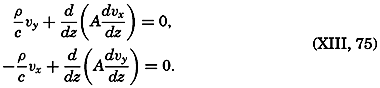
Assuming that the eddy viscosity is independent of depth, one can integrate the equations directly. Writing
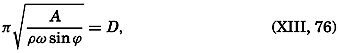
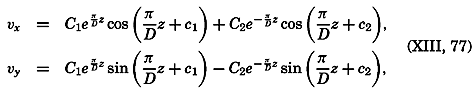
In this form the result is applicable to conditions in the Northern Hemisphere only, because in the Southern Hemisphere sin ϕ is negative, wherefore D is imaginary. In order to obtain a solution that is valid in the Southern Hemisphere, the direction of the position of the y axis must be reversed.
The solution takes the simplest form if the depth to the bottom is so great that one can assume no motion near the bottom, because then
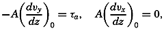
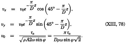
Therefore, the wind current is directed 45° cum sole from the direction of the wind. The angle of deflection increases regularly with depth, so that at the depth z = D the current is directed opposite to the surface current. The velocity decreases regularly with increasing depth, and at z= D is equal to e−x times the surface velocity, or one twenty-third of the value at the surface. By far the more important velocities occur above the depth z = D, and Ekman has therefore called this depth “the depth of frictional resistance.” It should be observed, however, that according to this solution the velocity of the wind current never becomes zero, but approaches zero asymptotically and is practically zero below z = D
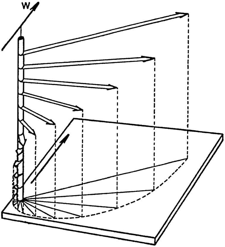
Schematic representation of a wind current in deep water, showing the decrease in velocity and change of direction at regular intervals of depth (the Ekman spiral). W indicates direction of wind.
A schematic representation of the pure wind current is given in fig. 121. The broad arrows represent the velocities at depths of equal intervals. Together they form a spiral staircase, the steps of which rapidly decrease in width as they proceed downward. Projected on a horizontal plane the end points of the vectors lie on a logarithmic spiral.
The average deflection of the wind current from the direction of the wind has been examined (Krümmel, 1911) and found to be about 45° cum sole from the wind direction, independent of latitude, in agreement with Ekman's theory.
The ratio between the velocity of the surface current, which Thorade has called the wind factor, depends upon the stress of the wind and upon the value of the eddy viscosity—that is, upon D. The stress of the wind is proportional to the square of the wind velocity, τa = 3.2 10−6W2 (p. 490), where the wind velocity, W, is measured in centimeters per second. Introducing this value into (XIII, 78), one obtains
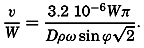
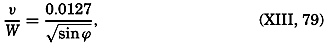
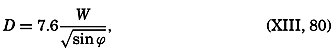
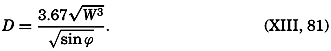
From equations (XIII, 76), (XIII, 80), and (XIII, 81), one obtains (see table 64)
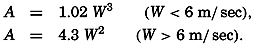
| Wind velocity (m/sec) | 2 | 4 | 6 | 8 | 10 | 15 | 20 |
| A (g/cm/sec) | 8 | 65 | (218) | 375 | 430 | 970 | 1720 |
Rossby (1932) and Rossby and Montgomery (1935) have developed a new theory of the wind currents by introducing an eddy viscosity that
According to Ekman's theory the angle should remain constant at 45°, and the wind factor, according to the empirical results that he made use of, should be equal to 0.025 in lat. 15° and 0.0136 in lat. 60°. Rossby and Montgomery point out that the wind factor depends upon the depth at which the wind current is measured. Their theoretical values apply to the current at the very surface, but wind currents derived from ships' logs will apply to a depth of 2 or 3 m, depending upon the draft of the vessel. At this depth, their theory gives a wind factor in better agreement with Ekman's value, and they show that their theoretical conclusions are in fair agreement with empirical results. However, the introduction of an eddy viscosity that decreases to zero at a lower limit of the wind-stirred layer is justifiable only if no other currents are present. In the presence of other currents, such as tidal currents or currents related to distribution of mass, the eddy viscosity characteristic of the total motion must be introduced, and the variation of this eddy viscosity probably depends more upon the stability of the stratification than upon the geometric distance from the free surface. A theory of the wind currents must take this fact into account, but such a theory cannot be developed until more is known of the actual character of the turbulence. At present, Ekman's classical theory appears to give a satisfactory approximation, especially because no observations are as yet available by means of which the results of a refined theory can be tested.
So far, it has been assumed that the depth of the water is great compared to the depth of frictional resistance. Ekman has also examined the wind currents in shallow water and has determined the constants in equations (XIII, 77) by assuming that at the bottom the velocity is zero. This analysis leads to the result that in shallow water the deflection of the surface current is less than 45° and that the turning with depth is slower. In very shallow water the current flows nearly in the direction of the stress at all depths.
The assumption of an eddy viscosity that is independent of depth is not valid, however, if the water is shallow, because the eddy viscosity must be very small near the bottom (p. 480), regardless of the character of the current. The effect of a decrease of the eddy viscosity toward the bottom is generally that the angle between wind and current becomes greater at all depths and that the current velocities become greater. This effect is illustrated by measurements of wind currents on the North Shelf in lat. 76°35′ N, long. 138°24′ E (Sverdrup, 1929), where the depth to the bottom was 22 m. From these observations, Fjeldstad (1929) found that the eddy viscosity could be represented by the formula
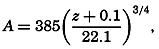
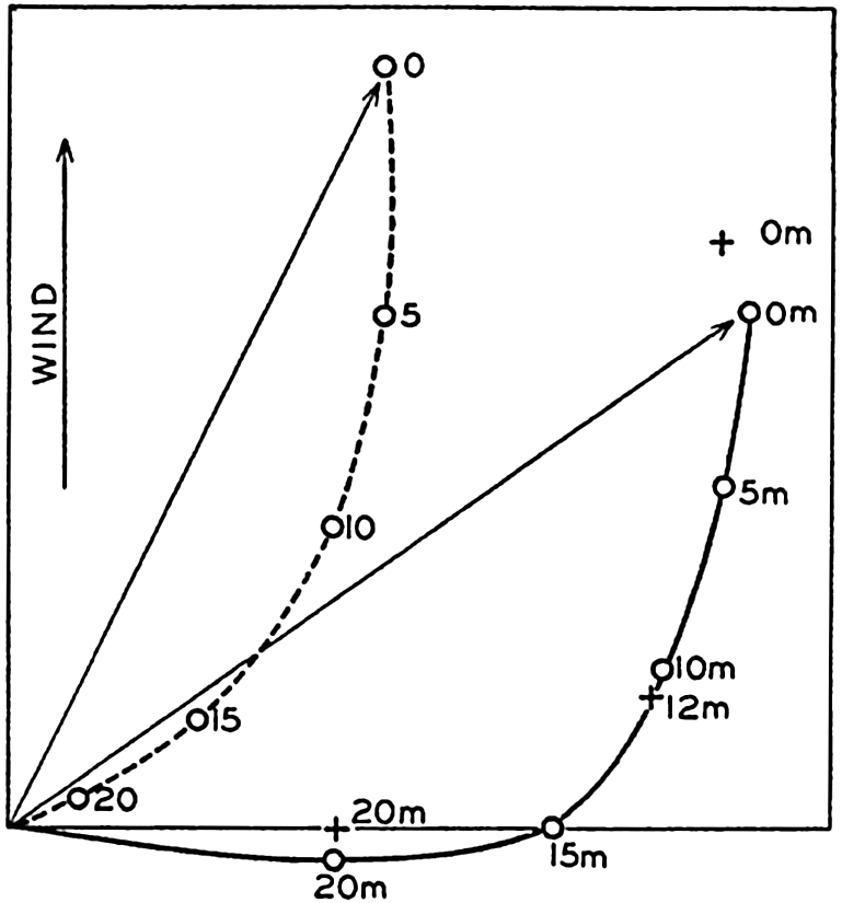
Wind current in shallow water assuming a constant eddy viscosity (dashed curve) or an eddy viscosity which decreases towards the bottom (full-drawn curve). Observed currents indicated by crosses.
The question of the time needed for establishing the assumed stationary conditions has also been examined by Ekman (1905), who has made use of a solution given by Fredholm for the case of a wind that suddenly begins to blow with a velocity which later remains constant. It is found that the motion will asymptotically approach a steady state. At each depth the end points of the velocity vectors, when represented as a function of time, will describe a spiral around the end point of the final velocity vector, the period of oscillation being 12 pendulum hours, corresponding to the period of oscillation by inertia movement (p. 438). The average velocity over 24 hours will be practically stationary from the very beginning, but the oscillations around the mean motion may continue for several days and may appear as damped motion in the circle of inertia.
Wind Currents in Water in Which the Density Increases with Depth. In the equations of motion which govern the wind current, the density enters explicitly, and it might therefore be expected
The rate at which a wind current penetrates toward greater depths will also depend upon the change of density with depth. Where an upper, nearly homogeneous layer of considerable thickness has already been developed by cooling from above and resulting vertical convection, the wind current will, in a short time, reach its normal state. Where a light surface layer has been developed because of heating or, in coastal areas, because of addition of fresh water, the wind current will first stir up the top layer and by mixing processes create a homogeneous top layer. When this layer is formed, the stability will be great at its lower boundary; there the eddy viscosity will be small and a further increase of the thickness of the homogeneous top layer will be effectively impeded, although the thickness may be much less than that of the layer within which normally a wind current should be developed. The further increase must be very slow, but no estimate can be given of the time required for the wind current to penetrate to the depths that it would have reached in homogeneous water. The gradual increase of the homogeneous top layer is shown schematically in fig. 123A.
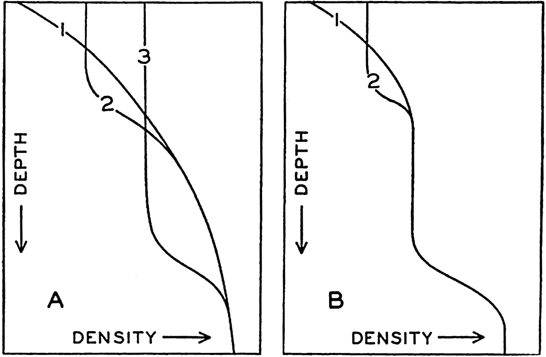
Effect of wind in producing a homogeneous surface layer demonstrated by showing progressive stages of mixing.
If the wind dies off, heating at the surface may again decrease the density near the surface, but as soon as the wind again starts to blow, a new homogeneous layer is formed near the surface, and consequently two sharp bends in the density curve may be present (fig. 123B).
If conclusions are to be drawn from the thickness of the upper homogeneous layer as to the depth to which wind currents penetrate, cases must be examined in which the wind has blown for a long time from the same direction and with nearly uniform velocity. In middle and high latitudes the wind current will reach its final state more rapidly in winter, when cooling takes place at the surface, than in summer, when heating takes place.
Transport and Energy Equations Applied to Wind Currents. The transport by wind currents across a vertical surface 1 cm wide is obtained by integration of the equations of motion, taking the boundary condition into account. In the open ocean, where the water is deep, the result is

If in homogeneous water the kinetic energy remains constant, the energy equation (XIII, 68) is reduced to

In Ekman's solution  , where ν0 is the velocity of the surface wind current, which deviates 45° from the direction of the wind. Because A is assumed to be constant, one obtains
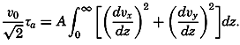
In nonhomogeneous water the complete energy equation has to be considered. The power of the wind stress on the surface must equal the work performed against the pressure gradients and the loss of energy by dissipation due to friction. This is only another way of stating that the wind currents are modified in stratified water, but so far the extent of modification has not been examined.
One of the characteristics of the modifications can be demonstrated as follows. The boundary condition must always be fulfilled (XIII, 65); that is,
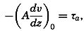
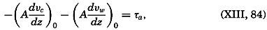
Effect of Friction on Bottom Currents. A current flows along the bottom if the isobaric surfaces are inclined near the bottom, and in this case the effect of friction cannot be neglected. The motion must be zero at the bottom, and directly over the bottom the eddy viscosity must increase rapidly with the distance from the bottom (see p. 480).
The equations of motion can easily be integrated if one assumes that the eddy viscosity is constant and that near the bottom the slope of the isobaric surfaces is independent of the distance from the bottom. The latter assumption implies that in the absence of friction the “gradient velocity,” Vi = − gci, is independent of the distance from the bottom. Placing the center of the coordinate system at the bottom, the positive y axis in the direction of the slope of the isobaric surfaces, and the z axis positive upward, one obtains
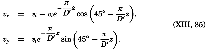
This solution, which was given also by Ekman, corresponds exactly to the solution which represents the wind current, and can be represented in a similar manner (see fig. 121, p. 493). Above the bottom the current first turns to the right and its velocity increases until, above the depth D′, which corresponds to the depth of frictional resistance, it practically attains the constant velocity vi. Projected on a horizontal plane, the end points of the velocity vectors lie on a logarithmic spiral.
This solution gives a first orientation as to the effect of friction near the bottom, but it cannot be expected that the solution will give a

The above considerations are valid if the depth of the water is greater than the thickness of the layer of frictional resistance. In shallow water, modifications are encountered which have been discussed by Ekman on the assumption of a constant eddy viscosity.
Secondary Effect of Wind Toward Producing Currents. Upwelling. In the open ocean the total mass transport by wind is equal to Cτa and is directed normal to the wind regardless of the depth to which the wind current reaches and regardless of the variation with depth of the eddy viscosity. This fact is of the greatest importance, because the transport of surface layers by wind plays a prominent part in the generation and maintenance of ocean currents. Boundary conditions and converging or diverging wind systems must, in certain regions, lead to an accumulation of light surface waters and, in other regions, to a rise of denser water from subsurface depths. Thus, the wind currents lead to an altered distribution of mass and, consequently, to an altered distribution of pressure that can exist only in the presence of relative currents. These processes will be illustrated by a few examples.
Consider in the Northern Hemisphere a coast line along which a wind blows in such a manner that the coast is on the right-hand side of an observer who looks in the direction of the wind (see fig. 124). At some distance from the coast the surface water will be transported to the right of the wind, but at the coast all motion must be parallel to the coast line. Consequently a convergence must be present off the coast leading to an accumulation of light water along the coast. This accumulation creates a relative field of pressure with which must be associated a current running parallel to the coast in the direction of the wind. Thus, the wind produces not only a pure wind current but also
Consider next a wind in the Northern Hemisphere which blows parallel to the coast, with the coast on the left-hand side. In this case the light surface water will be transported away from the coast and must, owing to the continuity of the system, be replaced near the coast by heavier subsurface water. This process is known as upwelling, and is a conspicuous phenomenon along the coasts of Morocco, Southwest Africa, California, and Peru (pp. 702 and 725). The upwelling also leads to changes in the distribution of mass, but now the denser, upwelled water accumulates along the coast and the light surface water is transported away from the coast. This distribution of mass again will give rise to a current that flows in the direction of the wind.
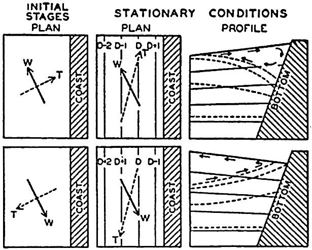
Schematic representation of effect of wind towards producing currents parallel to a coast in the Northern Hemisphere and vertical circulation. W shows wind direction, and T, direction of transport. Contours of sea surface shown by lines marked D, D + 1. … Top figures show sinking near the coast; bottom figures show upwelling.
The qualitative explanation of the upwelling was first suggested by Thorade (1909) and was developed by McEwen (1912). Recent investigations by Gunther (1936), Defant (1936b), Sverdrup (1930, 1938b), and Sverdrup and Fleming (1941) have added to the knowledge of the phenomenon, and have especially shown that water is drawn to the surface from depths not exceeding 200 to 300 m. Deep water does not rise to the surface, but an overturning of the upper layer takes place.
In spite of the added knowledge, it is as yet not possible to discuss quantitatively the process of upwelling or to predict theoretically the velocity and width of the coastal current that develops. It is probable that the tendency of the current is to break up in eddies, and that the forced vertical circulation limits the development of the current. Also, the wind that causes the upwelling does not, as a rule, blow with a steady velocity, and variations of the wind may greatly further the formation of eddies.
Figure 125 demonstrates the effect of winds from different directions on the currents off the coast of southern California in 1938. The charts show the geopotential topography of the sea surface relative to the 500-decibar surface, which in this case can be considered as nearly coinciding with a level surface. Arrows have been entered on the isolines, indicating that these are approximately stream lines of the surface currents.
In the absence of wind, one should expect a flow to the south or southeast, more or less parallel to the coast. In February, 1938 (fig. 125A), winds from the south or southwest had been blowing for some time. The light surface water had been carried toward the coast, and, consequently, a coastal current running north was present and was separated from the general flow to the south by a trough line, which probably represents a line of divergence. This inshore current to the north may not be an effect of the wind only, however, but may represent a countercurrent that develops when variable winds blow (p. 677).
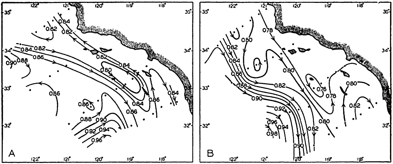
(A) Geopotential topography of the sea surface off southern California relative to the 500-decibar surface in February, 1938, after a period with westerly or southwesterly variable winds. (B) Topography and corresponding currents in June after a period with prevailing northwesterly winds.
In June, 1938 (fig. 125B) northwesterly winds had prevailed for several months and had carried the light surface water out to a distance of about 150 km from the coast, where the swift current followed the boundary between the light offshore water and the denser upwelled water. Within both types of water several eddies appear.
Similar considerations apply to conditions in the open ocean. Take the case of a stationary anticyclone in the Northern Hemisphere. Over the ocean the direction of the wind deviates but little from the direction of the isobars, so that the total transport of the wind will be nearly toward the center of the anticyclone. Light surface water will, therefore, accumulate near the center of the anticyclone, and a distribution of mass will be created that will give rise to a current in the direction of the
Mention has so far been made only of the direction of the wind, but the total transport depends also upon the square of the wind velocity and upon the latitude. In order to find the actual convergence due to wind, it is necessary, therefore, to take into account both the velocity and the latitude. An attempt in this direction has been made by Montgomery (1936), who finds that in the North Atlantic Ocean the region of maximum convergence lies to the south of the anticyclone. Further investigations of this nature are desirable.
Every wind system, whether stationary or moving, will create currents associated with the redistribution of mass due to wind transport. It is possible, furthermore, that within a moving wind system the distribution of mass does not become adjusted to the wind conditions, and that actual piling up or removal of mass may occur such as takes place in partly landlocked seas like the Gulf of Bothnia (p. 490). If this is true, slope currents reaching from the surface to the bottom develop, but they are of a local character and will soon be dissipated. One may thus expect that superimposed on the general currents will be irregular currents due to changing winds and, furthermore, eddies which are characteristic of the currents themselves and independent of wind action. A synoptic picture of the actual currents can therefore be expected to be highly complicated.
Conclusions as to Currents on the Basis of Tonguelike Distribution of Properties
Where horizontal differences in density are so small that differences in computed anomalies of distances between isobaric surfaces become doubtful, conclusions as to currents are often drawn from tonguelike distribution of properties, especially of temperature and salinity. In such cases, it is necessary to distinguish between tongues in a horizontal plane and those in a vertical section.
As a rule a tonguelike distribution in a horizontal plane can be interpreted by means of the dynamic considerations that have been presented. If a tongue of low temperature is present, as shown in fig. 126, one can assume in most cases that the water of the lowest temperature also has the highest density and, in accordance with the rule that in the Northern Hemisphere the water of the highest density must be found on the left-hand side of the current, arrows representing the approximate direction of flow can be entered. In the example shown in fig. 126 the flow to the northwest on the coastal side of the tongue of cold water was confirmed by results of drift-bottle experiments (Sverdrup and Fleming, 1941). Thus, the stream lines tend to follow the contour lines of the tongues.
If the dynamics of the system were not borne in mind, one might assume that the spread of the water would be jetlike and that the axes of the jet currents would coincide with the tongues of low or high temperatures, as indicated by the open arrows in fig. 126. Such an interpretation, however, would neglect the effect of horizontal pressure gradients and therefore would be in disagreement with the character of the acting forces. These conclusions will be somewhat modified by a consideration of the effect of friction, and they may not be valid at the sea surface, where external factors may contribute toward maintaining the temperature distribution.
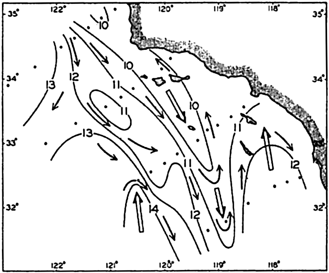
Tonguelike distribution of temperature at a depth of 50 m off southern California in May, 1937. Solid arrows indicate direction of flow according to the geopotential topography of the sea surface; open arrows show the axes of the tongues.
Consider next a vertical section in which a tonguelike distribution of temperature and salinity appears (fig. 127). In this case the tongue may indicate horizontal flow in the direction of the tongue, and such flow may no longer be in conflict with the dynamics of the system. However, if only horizontal motion occurs, processes of mixing must be of importance to the development of the tongue, because the properties of the mass in a moving volume are changing in the direction of flow, and in the subsurface layers such changes can be due only to mixing (p. 158).
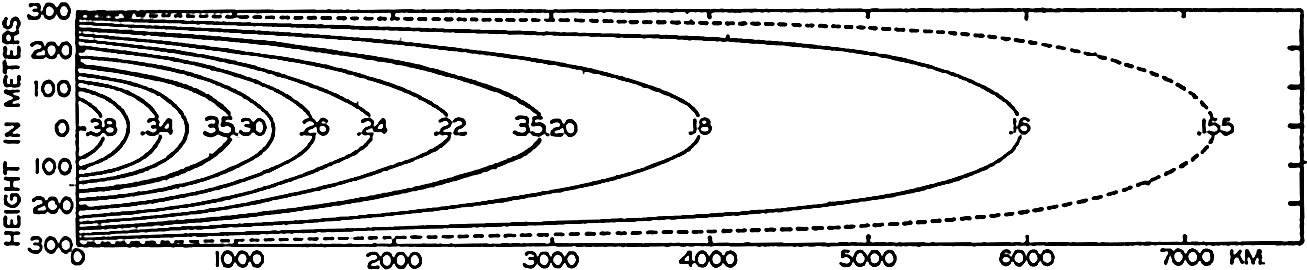
Tonguelike distribution of salinity in a vertical section corresponding to given boundary conditions and given values of velocity and eddy diffusion. See text.
Defant (1929b) and Thorade (1931) have examined analytically the relation between the velocity and the effect of vertical mixing. Under stationary conditions the equation (p. 159)
Equation (XIII, 86) can be solved if A/ρ is supposed to be constant and a number of simple assumptions are introduced. Consider, for instance, a horizontal current of uniform velocity, ν, in a layer of thickness 2h, flowing between z = +h and z = − h (see fig. 127). Assume that at x = 0 the distribution of the property is given by the equation
Figure 127 shows an example of such a distribution which has been prepared by Defant after the introduction of numerical values of s0, Δs, and h and by assuming that A/ν = 2. The solution presupposes certain boundary conditions that are not specified here. Transport of the property into the volume must take place through the surface x = 0, and transport out of the volume must take place through the other boundary surfaces. In these circumstances, it is necessary to assume that certain physical processes maintain the constant value s = s0 along the horizontal boundaries.
As shown by Thorade (1931), equation (XIII, 86) can be integrated on many different assumptions, and different types of tongues can be derived. It is particularly interesting to observe that on certain assumptions the tongue is found to curve up or down, although horizontal flow is assumed, and that the axis of the tongue need not coincide with an axis of maximum velocity. In fig. 127, uniform velocity was supposed, but the tonguelike distribution of the property may create the erroneous impression that the velocity is at a maximum along the center line of the tongue. In view of these results, it is necessary to exercise great care when drawing conclusions as to currents from tonguelike distribution.
Defant (1936a) has made use of equation (XIII, 86) in an improved form in order to compute the ratio A/ν directly from oceanographic data. Considering that along the bottom the motion cannot be horizontal, but must follow the slope of the bottom and that, even at some distance from the bottom, the motion may deviate from the horizontal, Defant writes
It has so far been assumed that horizontal mixing can be disregarded, but a tonguelike distribution can equally well be brought about by horizontal and vertical mixing and by horizontal flow and vertical mixing. If a given distribution in a vertical plane is maintained only by processes of mixing in horizontal and vertical directions, equation (XIII, 86) must be replaced by
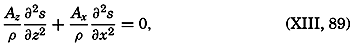
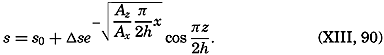
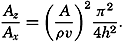
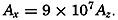
The “core method,” which Wüst has introduced (p. 146) and used successfully in studying the deep-water flow in the Atlantic, does not contain any assumption as to the character of the mixing, and is well suited therefore for giving a qualitative picture of the spreading of certain water types.
Thermodynamics of Ocean Currents
The preceding description of the effect of the wind, especially the discussion of the secondary effect of the wind in producing currents in stratified water, may leave the impression that the wind is all-important to the development of the ocean currents and that thermal processes can be entirely neglected. Such an impression would be very misleading, however. In discussing the secondary effect of the wind, it was repeatedly mentioned that the development of the currents caused by a redistribution of mass by wind transport would be checked partly by mechanical processes and partly by thermal processes. Surface waters that were transported to higher latitudes would be cooled, and thus a limit would be set to the differences in density that could be attained. Upwelling water would be heated when approaching the surface, and at a certain vertical velocity a stationary temperature distribution would be established at which the amount of heat absorbed in a unit volume would exactly balance the amounts lost by eddy conduction and by transport of heat through the volume by vertical motion. The establishment of a stationary temperature distribution within upwelling water would check the effect of upwelling on the horizontal distribution of density.
The above examples serve to emphasize the importance of the thermal processes in the development of the currents, but an exact discussion of the thermodynamics of the ocean is by no means possible. So far, the principles of thermodynamics have found very limited application to oceanographic problems, but this statement does not mean that the thermal processes are unimportant compared to the mechanical.
Thermal Circulation. The term “thermal circulation” will be understood to mean a circulation that is maintained by heating a system in certain regions and by cooling it in other regions. The character of the thermal circulation in the ocean and in the atmosphere has been discussed by V. Bjerknes and collaborators (1933). Their conclusions can be stated as follows: If within a thermal circulation heat shall be transformed into mechanical energy, the heating must take place under higher pressure and the cooling under lower pressure. Such a thermodynamic
In the ocean, “higher pressure” can generally be replaced by “greater depth,” and “lower pressure” by “smaller depth.” Applied to the ocean the theorem can be formulated as follows: If within a thermal circulation heat shall be transformed into mechanical energy, the heating must take place at a greater depth than the cooling.
This theorem was demonstrated experimentally by Sandström previous to its formulation by Bjerknes. In one experiment, Sandström placed a “heater” at a certain level and a “cooler” at a lower level in a vessel filled with water of uniform temperature. The heater consisted of a system of tubes through which warm water could be circulated, and the cooler consisted of a similar system through which cold water could be circulated. When warm and cold water were circulated through the pipes, a system of vertical convection currents developed and continued until the water above the heater had been heated to the temperature of the circulating warm water, and the water below the cooler had been cooled to the temperature of the circulating cold water. When this state had been reached and a stable stratification had been established, with temperature decreasing downward, all motion ceased.
In a second experiment, Sandström placed the cooling system above the heating system. In this case the final state showed a circulation with ascending motion above the heating unit and descending motion below the cooling unit. Thus, a stationary circulation was developed, because the heating took place at greater depth than the cooling.
From these experiments and from Bjerknes' theorem, it is immediately evident that in the oceans conditions are very unfavorable for the development of thermal circulations. Heating and cooling take place mainly at the same level—namely, at the sea surface, where heat is received by radiation from the sun during the day when the sun is high in the sky, or lost by long-wave radiation into space at night or when the sun is so low that the loss is greater than the gain and heat is received or lost by contact with air.
Because heating and cooling take place at the surface, one might expect that no thermal circulation can develop in the sea, but this is not true. Consider a vessel filled with water. Assume that heating at the surface takes place at the left-hand end, and that towards the right-hand end the heating decreases, becoming zero at the middle of the vessel. Beyond the middle, cooling takes place, and reaches its maximum at the other end. Under these conditions the heated water to the left will have a smaller density than the cooled water to the right, and will therefore spread to the right. Owing to the continuity of the system, water must rise near the left end of the vessel and sink near the right
This circulation is quite in agreement with Bjerknes' theorem, because at the surface the water that flows from left to right is being cooled, since it flows from a region where heating dominates into a region where cooling is in excess. During the return flow, which takes place at some depth below the surface, the water is, on the other hand, being warmed by conduction, because it flows from a region of lower temperature to a region of higher temperature. Thus the circulation is such that the heating takes place at a greater depth than the cooling. This circulation, however, cannot become very intensive, particularly because the heating within the return flow must take place by the slow processes of conduction.
If the oceanic circulation is examined in detail, many instances are found in which the vertical circulation caused by the wind is such that the thermal machine runs in reverse, meaning that mechanical energy is transformed into heat, thus checking the further development of the wind circulation. When upwelling takes place, the surface flow will be directed from a region of low temperature to a region of high temperature, and the subsurface flow will be directed from high to low temperature. The thermal machine that is involved will consume energy and thus counteract a too-rapid wind circulation. In the Antarctic the thermal circulation will be directed at the surface from north to south and will counteract the wind circulation, which will be directed from south to north. On the other hand, systems are found within which the thermal effect tends to increase the wind effect and within which the increase of the circulation must be checked by dissipation of kinetic energy.
The Thermohaline Circulation. So far, only thermal circulations have been considered, but it must be borne in mind that the density of the water depends on both its temperature and its salinity, and that in the surface layers the salinity is subject to changes due to evaporation, condensation, precipitation, and addition of fresh water from rivers. In the open ocean the changes in density are determined by the excess or deficit of evaporation over precipitation. These changes in density may be in the same direction as those caused by heating and cooling, or they may be in opposite directions. When examining the circulation that arises because of the external factors influencing the density of the surface waters, one must take changes of both temperature and salinity into account, and must consider not the thermal but the thermohaline circulation. Bjerknes' theorem is then better formulated as follows:
If thermal and haline circulations are separated, it is found that in some instances they work together and that in others they counteract each other. The greatest heating takes place in the equatorial region, where, owing to excess precipitation, the density is also decreased by reduction of the salinity. In the latitudes of the subtropical anticyclones the heating is less, and, in addition, the density of the water is increased by excess evaporation. Between the Equator and the latitudes of the subtropical anticyclones, conditions are therefore favorable for the development of a strong thermohaline circulation. North and south of these latitudes the haline circulation will, however, counteract the thermal, because the density is decreased by excess precipitation but increased by cooling. A weak thermohaline circulation might be expected there.
In the absence of a wind system, one might expect at the surface a slow thermohaline circulation directed from the Equator to the poles and directed at some subsurface depth in the opposite direction. This circulation would be modified by the rotation of the earth and by the form of the ocean basins, but nothing can be said as to the character of the system of currents that would develop under such conditions. It is probable, however, that the existing current system bears no similarity to the one that would result from such a thermohaline circulation, but is mainly dependent upon the character of the prevailing winds and upon the extent to which the circulation maintained by the wind is checked by the thermal conditions. In other words, the wind system tends to bring about a distribution of density that is inconsistent with the effect of heating and cooling, and the actual distribution approaches a balance between the two factors. These two factors—the wind and the process of heating and cooling—are variable, however, in time and space, for which reason a stationary distribution of density with accompanying stationary currents does not exist. Only when average conditions over a long time and a large area are considered can they be regarded as stationary.
Vertical Convection Currents. The thermohaline circulation is of small direct importance to the horizontal current, but is responsible mainly for the development of vertical convection currents. Wherever the density of the surface water is increased so much by cooling or evaporation that it becomes greater than the density of the underlying strata, the surface water must sink and must be replaced by water from some subsurface depth. The vertical currents that arise in this manner are called vertical convection currents. They are irregular in character and
The depth to which vertical convection currents penetrate depends upon the stratification of the water. A mass of surface water, the density of which has been increased by cooling or evaporation, sinks until it meets water of equal density. If mixing with neighboring water masses takes place, it sinks to a lesser depth. When vertical convection currents have been active for some time, an upper layer of homogeneous water is formed, the thickness of which depends upon the original stratification of the water, the intensity of the convection currents, and the time the process has lasted. Thus, an upper homogeneous layer can be formed in two different ways: either by the mechanical stirring due to wind, or by the effect of the thermohaline vertical convection currents.
The vertical convection currents are, as a rule, of greater importance in higher latitudes. In latitudes where an excess of evaporation is found, the heating of the surface is often so great that the decrease of the surface density by heating more than balances the increase by evaporation. In these circumstances the surface salinity will be greater than the salinity at a short distance below the surface. The formation of deep and bottom water by vertical convection currents is dealt with elsewhere (p. 138).
Bibliography
Bjerknes, V., J. Bjerknes, H. Solberg, T. Bergeron. 1933. Physikalische Hydrodynamik. Berlin. Julius Springer. 797 pp., 1933.
Bowie, William. 1936. “The place of geodesy in geophysical research” . Amer. Geophys. Un., Trans., p. 15–20, 1936.
Defant, A.1929a. “Dynamische Ozeanographie” . Einführing in der Geophysik, 3, 222 pp.Berlin. 1929.
Defant, A.1929b. Stabile Lagerung ozeanischer Wasserkörper und dazu gehorige Stromsysteme. Berlin, Universität, Institut f. Meereskunde, Veröff. N.F., A. Geogr.-naturwiss. Reihe, Heft 19, 33 pp., 1929.
Defant, A.1932. “Die Gezeiten und inneren Gezeitenwellen des Atlantischen Ozeans” . Deutsche Atlantische Exped. Meteor1925–1927, Wiss. Erg., Bd. 7, 1 Teil, 318 pp., 1932.
Defant, A.1936a. “Ausbreitungs- und Vermischungsvorgänge im Antarktischen Bodenstrom und im Subantarktischen Zwischenwasser” . Deutsche Atlantische Exped. Meteor1925–1927, Wiss. Erg., Bd. 6, 2 Teil Lief. 2, p. 55–96, 1936.
Defant, A.1936b. “Das Kaltwasserauftriebsgebiet vor der Küste Südwestafrikas” . Länderkundliche Forschung, Festschrift Norbert Krebs zur Vollendung des 60. Lebensjahres dargebracht, p. 52–66, 1936.
Defant, A.1940. “Die ozeanographischen Verhältnisse während der Ankerstation des Altair am Nordrand des Hauptstromstriches des Golfstromsnördlich der Azoren” . Ann. d. Hydrogr. u. Mar. Meteor., November–Beiheft, 4. Lief., 35 pp., 1940.
Defant, A.1941. “Die absolute Topographie des physikalischen Meeresniveaus und der Druckflächen, sowie die Wasserbewegungen im Atlantischen Ozean” . Deutsche Atlantische Exped. Meteor1925–1927, Wiss. Erg., Bd. VI, 2 Teil, 5. Lief., p. 191–260, 1941.
Defant, A., and Bj. Helland-Hansen. 1939. “Bericht über die ozeanographischen Untersuchungen im zentralen und östlichen Teil des Nordatlantischen Ozeans im Frühsommer 1938 (Internationale Golfstrom-Expedition)” . Preuss. Akad. d. Wissenschaften, Abhandl., Jahrg. 1939, Phys.-math. Klasse, Nr. 5, 64 pp., 1939.
Dietrich, Günter. 1937a. “Die dynamische Bezugsfläche, ein Gegenwarts-problem der dynamischen Ozeanographie.” Ann. d. Hydrogr. u. Mar. Meteor., Bd.65, pp. 506–19, 1937.
Dietrich, Günter. 1937b. Die Lage des Meeresoberfläche im Druckfeld von Ozean und Atmosphäre mit besonderer Berücksichtigung des westlichen Nordatlantischen Ozeans und des Golfs von Mexico. Berlin, Universität, Institut f. Meereskunde, Veröff., N. F., A. Geogr.-naturwiss. Reihe, Heft 33, 52 pp., 1937.
Ekman, V. Walfrid. 1902. “Om jordrotationens inverkan på vindströmmar i hafvet.” Nyt. Mag. f. Naturvid., v. 40, 1902. Kristiania.
Ekman, V. Walfrid. 1905. “On the influence of the earth's rotation on ocean currents.” Ark. f. Mat. Astr. och Fysik. K. Sv. Vet. Ak., Stockholm, 1905–06, v. 2, no. 11, 1905.
Ekman, V. Walfrid. 1923. “Über Horizontalzirkulation bei winderzeugten Meeresstromungen” . Arkiv. f. Mat. Astr. o. Fys., v. 17, no. 26, 1923. Stockholm.
Ekman, V. Walfrid. 1927. Meeresströmungen. Handbuch d. physikalischen u. technischen Mechanik, Bd. 5, Lief 1, p. 177–206, 1927.
Ekman, V. Walfrid. 1929. “Über die Strommenge der Konvektiönsstrome im Meere.” Lunds Univ. Arsskr., N. F., Afd. 2, v. 25, nr. 6, Lund u. Leipzig, 1929.
Ekman, V. Walfrid. 1932. “Studien zur Dynamik der Meeresströmungen” . Gerlands Beitr. z. Geophysik, Bd. 36, p. 385–438. Leipzig. 1932.
Ekman, V. Walfrid. 1939. “Neuere Ergebnisse und Probleme zur Theorie der Konvektionsströme im Meere” . Gerlands Beitr. z. Geophysik, Suppl. Bd. 4, Ergebn. d. kosmischen Physik IV, Physik d. Hydro- u. Lithosphäre, 74 pp., 1939. Leipzig.
Ekman, V. Walfrid, and Bj. Helland-Hansen. 1931. “Measurements of ocean currents (Experiments in the North Atlantic).” Kungl. fysiografiska Sallskapet i Lund Förhandlingar, v. 1, no. 1, 1931.
Fjeldstad, J. E.1929. “Ein Beitrag zur Theorie der winderzeugten Meeresströmungen.” Gerlands Beitr. z. Geophysik, Bd. 23, 1929.
Fjeldstad, J. E.1933. Wärmeleitung im Meere.Geofysiske Publikasjoner, v. 10, no. 7, 20 pp., 1933. Oslo.
Fjeldstad, J. E.1936. “Results of tidal observations. Norwegian North Polar Exped. with the Maud 1918–1925.” Sci. Results, v. 4, no. 4, 88 pp., 1936.
Gunther, E. R.1936. “A report on oceanographical investigations in the Peru coastal current” . Discovery Repts., v. 13, p. 109–275, 1936.
Gustafson, T., and B. Kullenberg. 1936. “Untersuchungen von Trägheits-strömungen in der Ostsee.” Sv. Hydr.-Biol. Komm. Skr., Ny Ser. Hydr., no. 13, 28 pp., 1936.
Helland-Hansen, Bj.1934. The Sognefjord section. p. 257–274 in James Johnstone Memorial Volume.Liverpool. Univ. Press, 348 pp., 1934.
Hidaka, K.1940. “Absolute evaluation of ocean currents in dynamical calculations” . Imperial Acad. Japan, Proc., v. 16, p. 391–393, 1940. Tokyo.
Iselin, C. O'D.1936. “A study of the circulation of the western North Atlantic” . Papers in Physical Oceanogr. and Meteor., v. 4, no. 4, 101 pp., 1936.
Jacobsen, J. P.1913. “Beitrag zur Hydrographie der dänischen Gewässer.” Komm. f. Havunders. Medd., Ser. Hydr., v. 2, no. 2, 94 pp., 1913. Copenhagen.
Jacobsen, J. P.1930. “Remarks on the determination of the movement of the water and the intermixing of the watersheets in a vertical direction.” Conseil Perm. Internat. p. l'Explor. de la Mer, Rapp. et Proc.-Verb., v. 64, p. 59–68, 1930.
Jacobsen, J. P., and A. J. C. Jensen. 1926. “Examination of hydrographical measurements from the research vessels Explorer and Dana during the summer of 1924.” Conseil Perm. Internat. p. l'Explor. de la Mer, Rapp. et Proc.-Verb., v. 39, p. 31–84, 1926.
Jakhelln, A.1936. The water transport of gradient currents.Geofysiske Publikasjoner, v. 11, 14 pp., 1936.
Krümmel, O.1911. Handbuch der Ozeanographie. v. 2, Stuttgart, Engelhorn, 764 pp., 1911.
La Fond, Eugene C.1939. “Variations of sea level on the Pacific coast of the United States.” Jour. Marine Research, v. 2, p. 17–29, 1939.
Lamb, H.1932. Hydrodynamics. London. Cambridge Univ. Press. 6th ed., 748 pp., 1932.
Lek, Lodewijk. 1938. Die Ergebnisse der Strom- und Serienmessungen. Snellius Exped. in the eastern part of the Netherlands East-Indies 1929–1930, v. 2, pt. 3, 169 pp., 1938.
McEwen, George F.1912. “The distribution of ocean temperatures along the west coast of North America deduced from Ekman's theory of the upwelling of cold water from the adjacent ocean depths.” Intern. Revue ges. Hydrobiol. u. Hydrogr., Bd. 5, p. 243–286, 1912.
McEwen, George F.1919. “Ocean temperatures, their relation to solar radiation and oceanic circulation.” Scripps Inst. Biol. Res. Misc. Studies in Agric. and Biol., SemicentennialPub. Univ. Calif., 1868–1918, p. 335–421, 1919.
Montgomery, R. B.1936. “Transport of surface water due to the wind system over the North Atlantic.” Papers in Physical Oceanogr. and Meteorol., v. 4, no. 3, p. 23–30, 1936.
Montgomery, R. B.1938. “Fluctuations in monthly sea level on eastern U. S. coast as related to dynamics of western North Atlantic Ocean.” Jour. Marine Research, v. 1, p. 165–185, 1938.
Montgomery, R. B.1939. “Ein Versuch den vertikalen und seitlichen Austausch in der Tiefe der Sprungschicht im äquatorialen Atlantischen Ozean zu bestimmen” . Ann. d. Hydrogr. u. Mar. Meteor., Bd. 67, p. 242–246, 1939.
Montgomery, R. B., and E. Palmén.1940. “Contribution to the question of the Equatorial Counter Current.” Jour. Marine Research, v. 3, p. 112–133, 1940.
Neumann, Gerhard. 1940. “Die ozeanographischen Verhältnisse an der Meeresoberfläche im Golfstromsektor nördlich und nordwestlich der Azoren.” Ann. d. Hydrogr. u. Mar. Meteor., Beiheft sum Juniheft, 1. Lief., 87 pp., 1940.
Palmén, E., and E. Laurila. 1938. “Über die Einwirkung eines Sturmes auf den hydrographischen Zustand im nordlichen Ostseegebiet” . Soc. Sci. Fen. Com. Phys.-Mat., v. 10, no. 1, 53 pp., 1938. Helsingfors.
Parr, A. E.1936. “On the probable relationship between vertical stability and lateral mixing processes.” Conseil Perm. Internat. p. l'Explor. de la Mer, Journal du Conseil, v. 11, p. 308–313, 1936.
Rossby, C.-G.1932. “A generalization of the theory of the mixing length with applications to atmospheric and oceanic turbulence.” Papers in Physical Oceanogr. and Meteorol., v. 1, no. 4, 36 pp., 1932.
Rossby, C.-G.1936a. “Dynamics of steady ocean currents in the light of experimental fluid mechanics.” Papers in Physical Oceanogr. and Meteorol., v. 5, no. 1, 43 pp., 1936.
Rossby, C.-G.1936b. “On the frictional force between air and water and on the occurrence of a laminar boundary layer next to the surface of the sea.” Papers in Physical Oceanogr. and Meteor., v. 4, no. 3, 20 pp., 1936.
Rossby, C.-G., and R. B. Montgomery. 1935. “The layer of frictional influence in wind and ocean currents.” Papers in Physical Oceanogr. and Meteorol., v. 3, no. 3, 101 pp., 1935.
Rouse, Hunter. 1938. Fluid mechanics for hydraulic engineers. New York. McGraw-Hill, 422 p., 1938.
Sandström, J. W., and B. Helland-Hansen. 1903. “Über die Berechung von Meeresströmungen.” Reports on Norwegian Fishery and Marine Investigations. Bd. 2, Nr. 4, 43 pp., 1903. Bergen.
Seiwell, H. R.1935. “The distribution of oxygen in the western basin of the North Atlantic.” Papers in Physical Oceanogr. and Meteorol., v. 3, no. 1, 86 pp., 1935.
Seiwell, H. R.1938. “Application of the distribution of oxygen to the physical oceanography of the Caribbean region.” Papers in Physical Oceanogr. and Meteorol., v. 6, no. 1, 60 pp., 1938.
Seiwell, H. R.1942. “An analysis of vertical oscillations in the southern North Atlantic.” Amer. Phil. Soc., Proc., v. 85, p. 136–158, 1942.
Smith, Edward H.1926. A practical method for determining ocean currents. U. S. Coast Guard, Bull.no. 14, 50 pp., 1926.
Suda, K.1936. “On the dissipation of energy in the density current (2nd paper).” Geophys. Mag., v. 10, p. 131–243, 1926. Tokyo.
Sverdrup, H. U.1926. Dynamic of tides on the North Siberian Shelf. Results from the Maud Expedition.Geofysiske Publikasjoner, v. 4, no. 5, 75 pp., 1926.
Sverdrup, H. U.1929. “The waters on the North Siberian Shelf.” Norwegian North Polar Exped. with the Maud 1918–1925, Sci. Results, v. 4, no. 2, 131 + 175 pp., 1929.
Sverdrup, H. U.1930. “Some oceanographic results of the Carnegie's work in the Pacific–-The Peruvian Current.” Amer. Geophys. Un., Trans., p. 257–264. 1930.
Sverdrup, H. U.1933. “Narrative and oceanography of the Nautilus Expedition, 1931.” Papers in Physical Oceanogr. and Meteorol., v. 2, no. 1, 63 pp., 1933.
Sverdrup, H. U.1938a. “On the explanation of the oxygen minima and maxima in the oceans. Conseil Perm. Internat. p. l'Explor. de la Mer” , Journal du Conseil, v. 13, no. 2, p. 163–172, 1938.
Sverdrup, H. U.1938b. “On the process of upwelling.” Jour. Marine Research, v. 1, p. 155–164, 1938.
Sverdrup, H. U.1939a. “Lateral mixing in the deep water of the South Atlantic Ocean.” Jour. Marine Research, v. 2, p. 195–207, 1939.
Sverdrup, H. U.1939b. “On the influence of stability and instability on the wind profile and the eddy conductivity near the ground.” Fifth Internat. Congr. Applied Mech., Trans., p. 369–372, 1939.
Sverdrup, H. U., and R. H. Fleming. 1941. “The waters off the coast of southern California, March to July, 1937” . Scripps Inst. Oceanogr., Bull., v. 4, p. 261–378, 1941.
Sverdrup, H. U., and Staff. 1942. “Oceanographic observations on the E. W. Scripps cruises of 1938.” Scripps Inst. Oceanogr., Records of Observationsv. 1, no. 1, 63 pp., 1942.
Taylor, G. I.1931. “Internal waves and turbulence in a fluid of variable density. Conseil Perm. Internat. p. l'Explor. de la Mer” , Rapp. et Proc.-Verb., v. 76, p. 35–43, 1931.
Taylor, G. I.1932. “The transport of vorticity and heat through fluids in turbulent motion.” Royal Soc. London, Proc., Ser. A, v. 135, p. 685–701, 1932.
Thorade, H.1909. “Über die Kalifornische Meeresströmung.” Ann. d. Hydrogr. u. Mar. Meteor., Bd. 37, p. 17–34, 63–76, 1909.
Thorade, H.1914. “Die Geschwindigkeit von Triftströmungen und die Ekmansche Theorie.” Ann. d. Hydrogr. u. Mar. Meteor., Bd. 42, p. 379–91, 1914.
Thorade, H.1928. “Gezeitenuntersuchungen in der Deutschem Bucht der Nordsee.” Deutsche Seewarte, Archiv, Bd. 46, Nr. 3, p. 1–85, 1928. Hamburg.
Thorade, H.1931. “Strömung und Zungenförmige Ausbreitung des Wassers.” Gerlands Beitr. z. Geophysik, Bd. 34, p. 57–76, 1931. Leipzig.
Wattenberg, H.1935. “Kalkauflösung und Wasserbewegung am Meeresboden.” Ann. d. Hydrogr. u. Mar. Meteor., Bd. 63, p. 387–391, 1935.
Werenskiold, W.1937. “Die Berechnung von Meeresströmungen.” Ann. d. Hydrogr. u. Mar. Meteor., Bd. 65, p. 68–72, 1937.
Wüst, Georg. 1920. Die Verdunstung auf dem Meere.BerlinUniversität, Institut f. Meereskunde, N. F., A. Geogr.-naturwiss. Reihe, Heft 6, 95 pp., 1920.
Wüst, Georg. 1940. “Das Relief des Azorensockels und des Meeresbödens nordlich und nordwestlich der Azoren.” Ann. d. Hydrogr. u. Mar. Meteor., August-Beiheft, 2. Lief., 19 pp., 1940.