8. Use of Space
HOME RANGE
A home range estimate is built from a map of the points where an animal is known to have been. The points we know are but a tiny sample of the terrain that the animal might use, and a good deal of thought and theoretical discussion has been devoted to divining the best way to estimate the true home range from isolated points (e.g., the six models summarized in Kenward 1987). Researchers who take radiolocations only every few hours or days do not know how the animal traveled between points, and models that fill in empty spaces, such as “the minimum convex polygon,” are often used to connect points for home range estimation. Although following an animal all day, as we did in this study, generates a series of points, we know quite accurately where the animal went, so the points can be connected into a line describing its path. After following many species of mammals by continuous radio-tracking over the years, including squirrels, porcupines, ocelots, and spiny rats, I have come to the conclusion that home ranges, especially when they are also territories, are often highly irregular in outline, with odd hollows and protuberances. Thus, to estimate treeshrew home ranges, I have connected the outer points to form a minimum polygon, without enclosing large peripheral areas where I never recorded the animal to be. The home range outlines are therefore in many cases concave or spiky. The estimated ranges are smaller than they would be with the more standard convex polygon method, but the most important difference between
Home ranges are spatial projections of all the resource needs of individuals, and they thus hold whatever is needed by an animal at a particular time. For most mammals, it is best to compare only females to address ecological questions about home ranges—how much space is used by members of species with different diets? how far or long must individuals forage? how many can live in a hectare?—or other topics related to energetics. The reasons for this are straightforward: (1) females carry the energetic load of the production of offspring, so only the home ranges of females reflect the ecological baseline for reproduction, or fitness; (2) male travels and home ranges often reflect social, not ecological, motives, because the typical mammalian social organization is such that the agenda of males is not to use spatial resources efficiently but to acquire access to as many females as possible. As a main aim of this study was to try to put the reproductive system of treeshrews into an ecological context, I deliberately biased radio-tracking efforts heavily in favor of females. Moreover, adult males of most species were scarcer than females, and we caught fewer to radio-collar. Strategically, I first put radios on females and then tried to radio-tag the adult males that used the home areas of collared females. Ultimately, we followed twice as many females as males.
The crude home range values for forty-seven treeshrews followed by radio-tracking and one from trapping show high consistency between members of a species and sex (table 8.1). Because the values for animals tracked at Poring are close to those for the same species at Danum, and their behaviors were similar, data from both sites are treated together for species averages. Some treeshrews went off the edge of the trail system, beyond the reach of the receiver, so their ranges are known to be underestimates, while others were followed too briefly, so their ranges are incomplete (table 8.1). The distribution of total home range size as a function of numbers of points shows that for the most part there were adequate samples (home ranges with the most points were not the biggest ones) (fig. 8.1).
The mean home range sizes for species ranged from 1.5 ha to 10.5 ha (table 8.2). When these are related to body mass (fig. 8.2), it is evident that body size is a poor predictor of home range size: among females of the three smallest species, whose body weights differ by only 20 g,
| Species | Sex/No. | D max (m) | D min (m) | M/Day | Area (ha) | No. of Points |
|---|---|---|---|---|---|---|
| NOTE: D max = major axis (maximum diameter) of home range; D min = minor axis. Measured from maps of all compiled location points. -p = animals followed at Poring, (s) after animal number = subadult. M/day is the average of all complete days of tracking (N), excluding days where the animal was lost out of range or tracking was grossly curtailed by heavy rain. (*) animals whose home ranges were partly out of range (incomplete). | ||||||
| P. lowii | F96s | 268 | 200 | 995 (5) | 3.17 | 230 |
| F163s | 210 | 131 | 856 (8) | 1.93 | 230 | |
| F181 | 376 | 236 | 1,376 (7) | 6.41 | 288 | |
| T. minor | F70 | 261 | 103 | 1,032 (4) | 2.01 | 207 |
| F112-p | 124 | 109 | 667 (4) | 0.94 | 230 | |
| F294 | 193 | 139 | 854 (5) | 1.61 | 230 | |
| M91 | 224 | 124 | 866 (4) | 1.59 | 230 | |
| M126-p | 251 | 80 | 963 (3) | 1.27 | 151 | |
| T. gracilis | F67 | 419 | 417 | 1,765 (9) | 10.52 | 466 |
| F105-p | 660 | 191 | 1,339 (7) | 7.05 | 230 | |
| F173 | 500 | 271 | 1,452 (3) | 9.77 | 230 | |
| Mfoot | 561 | 344 | 2,015 (5) | 14.71 | 223 | |
| T. longipes | F56 | 492 | 275 | 2,602 (5) | 8.78 | 285 |
| F66* | 457 | 292 | 1,708 (3) | 8.31 | 230 | |
| F86s | 389 | 225 | 1,735 (4) | 5.68 | 230 | |
| F132-p | 580 | 211 | 1,442 (7) | 7.79 | 230 | |
| F133-p* | 590 | 216 | 810 (1) | 4.07 | 230 | |
| M64 | 404 | 282 | 2,480 (3) | 8.49 | 230 | |
| M73* | 469 | 409 | 9.60 | 230 | ||
| M79s | 569 | 138 | 2,111(2) | 7.55 | 121 | |
| M138-p* | 710 | 253 | 2,441 (2) | 9.15 | 230 | |
| M287* | 638 | 271 | 2,711 (1) | 9.96 | 117 | |
| T. montana | F148-p* | 243 | 118 | 1,376 (2) | 2.10 | 123 |
| F150-p | 218 | 196 | 781 (4) | 2.40 | 230 | |
| F154-p | 396 | 247 | 938 (4) | 3.09 | 230 | |
| M143-p | 218 | 177 | 971 (4) | 2.32 | 230 | |
| M144-p | 318 | 95 | 916 (4) | 1.48 | 230 | |
| M155-p | 235 | 5 | ||||
| T. tana | F54 | 272 | 156 | 1,054 (3) | 2.32 | 157 |
| F58 | 343 | 191 | 1,512 (4) | 4.02 | 230 | |
| F65 | 430 | 130 | 1,185 (3) | 2.68 | 230 | |
| F76 | 421 | 283 | 1,024 (7) | 5.63 | 230 | |
| F78* | 283 | 113 | 854 (3) | 1.94 | 230 | |
| F100 | 314 | 256 | 954 (4) | 4.82 | 230 | |
| F106-p | 271 | 109 | 897 (5) | 2.42 | 230 | |
| F109-p | 335 | 193 | 897 (15) | 3.97 | 230 | |
| F166 | 334 | 220 | 914 (3) | 3.65 | 230 | |
| F176 | 224 | 156 | 980 (4) | 2.14 | 230 | |
| F297 | 227 | 210 | 1,006 (3) | 2.50 | 230 | |
| MScar* | 320 | 235 | 1,584 (2) | 4.05 | 230 | |
| M7 | 336 | 221 | 970 (3) | 3.52 | 230 | |
| M55 | 424 | 200 | 1,327 (2) | 6.48 | 230 | |
| M62 | 330 | 247 | 792 (2) | 4.51 | 75 | |
― 127 ― T. tana | M63 | 444 | 338 | 1,470 (3) | 8.04 | 127 |
| M77 * | 621 | 201 | 1,451 (4) | 7.56 | 158 | |
| M111-p* | 455 | 241 | 1,363 (1) | 6.34 | 88 | |
| M167 | 317 | 199 | 1,045 (3) | 3.31 | 117 | |
| M168* | 276 | 220 | 1,218 (1) | 2.64 | 94 | |
| Species | N | D max (m) | SD | D min (m) | SD | Area (ha) | SD |
|---|---|---|---|---|---|---|---|
| P. lowii, all (F) | 3 | 284.7 | 84.3 | 189.0 | 53.4 | 3.84 | 2.3 |
| Adult female | 1 | 376.0 | 236 | 6.41 | |||
| T. minor, all | 5 | 210.6 | 55.1 | 111.0 | 22.3 | 1.48 | 0.4 |
| Female | 3 | 192.7 | 68.5 | 117.0 | 19.3 | 1.52 | 0.5 |
| Male | 2 | 237.5 | 19.1 | 102.0 | 31.1 | 1.43 | 0.2 |
| T. gracilis, all | 4 | 535.0 | 101.6 | 305.8 | 97.0 | 10.51 | 3.2 |
| Female | 3 | 526.3 | 122.6 | 293.0 | 114.6 | 9.11 | 1.8 |
| Male | 1 | 561.0 | 344.0 | 14.71 | |||
| T. longipes, all | 10 | 529.8 | 104.3 | 257.2 | 70.3 | 7.94 | 1.8 |
| Female | 5 | 501.6 | 84.7 | 243.8 | 37.1 | 6.93 | 2.0 |
| Male | 5 | 558.0 | 123.8 | 270.6 | 96.4 | 8.95 | 1.0 |
| T. montana, all | 5 | 271.3 | 71.5 | 166.6 | 61.1 | 2.28 | 0.6 |
| Female | 3 | 285.7 | 96.3 | 187.0 | 65.0 | 2.53 | 0.5 |
| Male | 2 | 257.0 | 53.5 | 136.0 | 58.0 | 1.90 | 0.6 |
| T. tana, all | 20 | 348.9 | 94.0 | 206.0 | 56.0 | 4.11 | 0.4 |
| Female | 11 | 314.0 | 68.4 | 183.4 | 56.8 | 3.28 | 1.2 |
| Male | 9 | 391.4 | 106.9 | 233.6 | 43.1 | 5.16 | 2.0 |
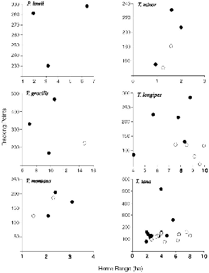
Fig. 8.1. Total number of radio-tracking location points recorded for each treeshrew followed and its home range in hectares. Females = black circles; males = open circles.
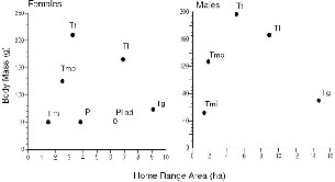
Fig. 8.2. Treeshrew home range areas as a function of body mass, means for each sex. For Ptilocercus lowii, the species mean includes two probable subadults; the open circle represents the adult, reproductive female F181.
SPEED AND DAILY DISTANCE TRAVELED
Paths traced by radio-tracking are straight lines between triangulated points, but animals actually zigzag, so recorded path lengths are minima and true distances moved must always be greater. One researcher has measured the difference between the real path of a small mammal and that given by radio-tracking. Guillotin (1982) followed spiny rats (Proechimys spp.) by sight and measured their exact itineraries to compare with radiolocation data. He found that the mean real path was 1.8 times longer than the telemetry-estimated one. Thus even “continuous” radio-tracking may largely underestimate path length. In addition, radiotracking does not register the vertical displacements of arboreal or scansorial species (perhaps equal to or greater than their horizontal travels). Animals thus travel much farther than we can measure by usual field
| Species | Distance (m) | Range (m) | SD | Rate,a (m/h) |
|---|---|---|---|---|
| aRate of movement is crudely estimated from mean m traveled ÷ (mean h active − mean h resting). | ||||
| b( ) = number of full-day samples. | ||||
| P. lowii, all (20)b | 1,073 | 568–1,613 | 295 | 124 |
| Adult female (7) | 1,376 | 1,012–1,613 | 37 | 131 |
| T. minor, all (20) | 871 | 558–1,234 | 175 | 83 |
| Female (13) | 851 | 558–1,234 | 200 | 80 |
| Male (7) | 908 | 779–1,057 | 120 | 87 |
| T. gracilis, all (24) | 1,654 | 722–2,522 | 474 | 151 |
| Female (19) | 1,559 | 722–2,240 | 457 | 145 |
| Male (5) | 2,015 | 1592–2,522 | 382 | 171 |
| T. longipes, all (28) | 1973 | 810–3,932 | 702 | 178 |
| Female (20) | 1800 | 810–3,932 | 744 | 165 |
| Male (8) | 2407 | 1,691–2,711 | 114 | 210 |
| T. montana, all (17) | 958 | 685–1,510 | 205 | 84 |
| Female (8) | 859 | 705–1,056 | 123 | 78 |
| Male (9) | 1047 | 685–1,510 | 230 | 89 |
| T. tana, all (74) | 1078 | 521–1,930 | 300 | 105 |
| Female (53) | 1009 | 577–1,682 | 256 | 97 |
| Male (21) | 1250 | 512–1,930 | 340 | 128 |
The rates at which treeshrew species normally moved varied by a factor of about 2, with T. longipes and T. gracilis in a class by themselves, moving faster than the others (table 8.3). The highest day's average was recorded for T. longipes F56, who on 26 October traveled 3.9 km, moving for 11.8 hours at the prodigious mean rate of 333 meters per hour. The rates in table 8.3 are averages throughout the day and all activities. When running quickly, T. longipes streaked through the forest at over 800 meters per hour (with a sweating researcher panting in distant pursuit).
Males of all species moved both faster and farther in a day than females, even when their home ranges were slightly smaller (T. minor, T. montana).
HOME RANGE SIZE AND ENERGETICS
Home range size has long been used as an index of bioenergetics. Simply put: “The size of the home range in mammals, accordingly, is determined by the rate of metabolism. A large mammal has a larger home range than a small mammal, because it uses more energy and, therefore, needs a greater area in which to find this energy” (McNab 1963: 136). As Mc-Nab showed in this early paper, and developed later (McNab 1983), there is a predictable relationship in mammals between body size, metabolic rate, diet class, and home range size. This idea makes intuitive sense and works generally, but within the log-log plots that demonstrate such trends is much scatter that looms large when plotted on linear scales (see fig. 8.2). This scatter may result from differences in diet or social behavior, especially if males are included. If only females are compared, it may result from the fine-tuned ecological differences in foraging habits that comprise the individual adaptations of species, as I shall argue below.
The connection between home range size and actual energy expenditure is indirect (as opposed to metabolic need). The amount of energy that an animal uses for daily activities, above its basal metabolic rate, should be somehow directly related to the actual distance that it travels, along with associated factors such as gait and terrain. The home range area, however, is largely a function of the directions that travel takes, or the shape of the path, and not necessarily its length. To look at this relationship, the mean distance that each tupai traveled per day can be plotted against its own home range size (fig. 8.3). This shows that the individuals of a species generally show consistency but that there are marked interspecific differences. The steeper the slope, and the higher the Y intercept, the greater the distance traveled per hectare of home range. Thus, at the extremes, a T. minor that travels 1,000 m per day has a home range of 2 ha, but a T. longipes that travels that distance has one of 5 ha. If a T. minor were to travel 2,000 m a day, its home range would only be 4 ha, but a T. gracilis that runs 2,000 m has a home range of nearly 15 ha.
If an animal zigzags, goes back on its path, or returns repeatedly to the same place, it may travel a long way within a small area. In a graphic example from the data (fig. 8.4), on one day T. minor M91 traveled 979 m within an area of 0.715 ha; and on another day T. gracilis Mfoot ran 1,592 m (his shortest recorded daily path) but covered 7.195 ha. The species means for the distance/area relationship show clearly that as home ranges become larger, daily path length increases at a much slower rate,
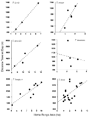
Fig. 8.3. The relationship between mean meters traveled per day and area of home range, for all individuals of each species. Note that scales are different.
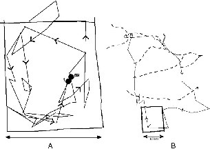
Fig. 8.4. Contrasting patterns of daily use of space, one complete day's movement. A, T. minor male M91, 7 December 1990, 39 location points, 974 m traveled, 0.72 ha covered. Square is a 1 ha quadrat of the grid of studyarea trails, circles are nest sites. B, T. gracilis Mfoot 31 July 1991, 41 location points, 1,592 m traveled (one of his shorter days), 7.20 ha covered. Square at bottom is the same quadrat shown in A. Heavy dashed lines are stream courses.
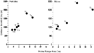
Fig. 8.5. Mean distance traveled per day by treeshrew species as a function of mean home range size, for each sex and species.
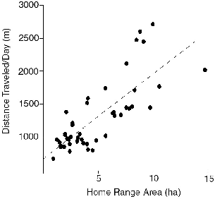
Fig. 8.6. The general relationship between mean meters traveled per day and area of home range, from data for all individual treeshrews (linear regression: m = 667.52 + 129.25 area).
Thus, although the home range of a female is a map of the distribution of the resources that she needs/uses during a particular time span, its area reflects the configuration of the daily foraging paths more than their absolute lengths. For males, the relationship between distance traveled and home area was similar to that for females of the same species (see fig. 8.5).
On the maps of daily movements, I also measured the area of the daily range, but it was evident that this calculation was both useless and misleading as an ecological descriptor: the real land use by an animal on a particular day is the narrow strip along its actual path. Daily ranges often were odd shapes, long and thin or curved. Connecting the points into a polygon always included areas that the animal went nowhere near, and deciding how to connect the points was highly subjective. The shape of the path, not its length, determined the daily area.
Another set of measurements often used in animal studies is the maximum and minimum diameters of the home range (see tables 8.1, 8.2). I
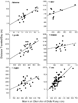
Fig. 8.7. the distance trveled during a day's activty as a function of the maximum diameter of the range for that day. Each point is one individual daily record.
PATTERNS OF TRAVEL AND DESTINATIONS
All Tupaia species ate fruit and invertebrates, and I assume that the daily travels of females were mostly directed toward finding one or the other of these commodities. Because I could rarely watch treeshrews, I had to assume that what I did see was typical of the overall activity that was hidden and infer from treeshrew movements what they might have been doing.
fruit trees
Fruit trees were the most evident specific destinations of treeshrew travels. A favored tree was visited repeatedly and could be the focal point of activity (chap. 4). Tupaia minor, T. gracilis, and T. longipes would intensively concentrate their activity around such trees. Because of their typically vast daily excursions, a focus of movements to a single destination at a fruit tree was most easily detected and unambiguous for T. gracilis and T. longipes (see fig. 4.1). T. tana were rarely so focused, but nevertheless they clearly aimed their itineraries to some fruit sources. T. montana was followed too briefly to evaluate its fruit foraging.
For T. minor, T. gracilis, and T. longipes, the use of fruit trees was in a loose way inversely correlated with the distance traveled in a day (table 8.4). There is too much variation for calculation of mean values, and there are few strictly comparable data sets (the same animal during the same month with and without a fruit tree), so I simply give the raw data. This shows that treeshrews usually traveled less far on days when they spent the most time at known fruit sources. This result can be viewed in two ways: either the time spent at fruit trees simply made less time available for other travel; or when fruit was an important food source, the distance required for foraging was smaller. One or both may be the case on particular days, but the result would seem to be that because treeshrews traveled less distance per day when feeding on some fruit species, they used less travel energy per day. The distance “saved” by eating fruit was up to 30 percent, compared to movements when no focal fruit tree was apparent.
other features of the environment
Treeshrews used the entire forest but preferred some areas over others. All terrestrial treeshrews at Danum Valley that had it in their home range spent
| Treeshrew | Month | No. of visits to Fruit | Hours at Fruit Tree | Distance/ Day (m) | Fruit |
|---|---|---|---|---|---|
| T. minor | |||||
| F112 | April | 7 | 6.44 | 678 | Myrisincease, Ficus |
| 5 | 4.74 | 667 | Myrsinaceae | ||
| 7 | 3.05 | 824 | Myrsinaceae | ||
| 3 | 2.16 | 617 | Myrsinaceae | ||
| 3 | 2.11 | 558 | Myrsinaceae | ||
| M126 | May | 7 | 4.65 | 666 | Ficus |
| 3 | 2.31 | 802 | Ficus | ||
| nr | nr | 1,057 | none | ||
| nr | nr | 1,030 | none | ||
| 4 | 1.24 | 913 | Parthenocissus | ||
| 2 | 0.91 | 979 | Parthenocissus | ||
| 1 | 0.62 | 1,234 | Parthenocissus | ||
| nr | nr | 1,048 | none | ||
| nr | nr | 1,002 | none | ||
| T. gracilis | |||||
| F105 | May | 1 | 4.21 | 722 | Ficus |
| 1 | nr | 878 | Ficus | ||
| 2 | nr | 1,060 | Ficus | ||
| nr | nr | 1,297 | none | ||
| August | 3 | 1.72 | 1,671 | Ficus | |
| 2 | 1.10 | 1,174 | Ficus | ||
| 1 | 1.00 | 1,461 | banana | ||
| 3 | 0.83 | 2,051 | Ficus | ||
| 2 | nr | 1,793 | Ficus | ||
| F67 | September | 2 | 2.60 | 2,240 | Dimocarpus |
| October | 3 | 4.84 | 1,982 | Dimocarpus | |
| 2 | 0.93 | 1,858 | Dimocarpus | ||
| 4 | 0.48 | 2,238 | Dimocarpus | ||
| F173 | July | 4 | 2.6 | 1,376 | Alangium |
| June | nr | nr | 1,919 | none | |
| nr | nr | 1,458 | none | ||
― 138 ― T.Longipes | |||||
| F132 | May | 1 | 5.80 | 997 | Ficus |
| 4 | 4.17 | 1816 | Ficus (2tress) | ||
| 6 | 3.84 | 1,669 | Ficus (2 trees) | ||
| 1 | 3.60 | 1,422 | Ficus (2 trees) | ||
| 2 | 0.73 | 1,170 | Ficus (2 trees) | ||
| nr | nr | 1,933 | none | ||
| F133 | May | 2 | 2.48 | 810 | Ficus |
| 4 | 2.14 | 1,118 | Ficus | ||
| nr | nr | 1,026 | none | ||
| F56 | October | 3 | 0.86 | 3,932 | Polyalthia |
| 2 | 0.17 | 2,821 | Polyalthia | ||
| F86 | March | 5 | 1.51 | 2,189 | Ficus |
| nr | nr | 2137 | none | ||
| M64 | December | 4 | 0.50 | 2,512 | Dialium |
| 4 | 0.46 | 2,673 | Dialium | ||
| 4 | nr | 2,255 | Dialium | ||
Tupaia tana had a characteristic habit of foraging along the banks of streams (fig. 8.8). This pattern was particularly marked on mornings after drenching nocturnal rains, when the animals would follow a stream closely, working their way along extremely slowly and steadily. For example, in the northwest leg of the path shown in figure 8.8A, F100 took an hour to travel 150 m. Only large treeshrews regularly behaved in this way, and I conjecture that they were hunting earthworms or crabs and crayfish (see chap. 5). Other terrestrial species often used watercourses as travel routes that they followed at normal speed. The paths of treeshrews often touched on streams, which they may have visited to drink water. At Poring the study area was largely on a ridge top without surface water, and all of the radio-collared T. tana frequently descended to
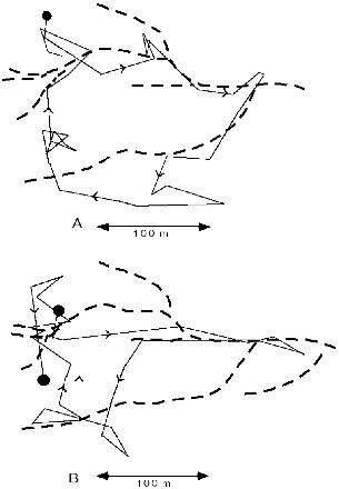
Fig. 8.8. Two sequential one-day itineraries of T. tana F100 that show use of stream courses (dashed lines). A, 13 June 91, after rain, 33 locations, 1,035 m traveled. On this day she ceased activity at only 1514 h. B, 14 June, 28 locations, 1043 m, activity ended at 1424 h. Note her use of different stream sections on the two days.
Treeshrews had particular pathways where they preferred to travel, and different terrestrial species used the same ones. All Tupaia species were attracted to treefalls and dense, dark, viny thickets, especially when these were in the damper forest understory, in small ravines and gullies. Treeshrews do not like to cross open spaces on the ground, so if there was a small log, root, or branch across a stretch of otherwise cleared trail, every individual would use it. Likewise, a dark area of low canopy over a trail was used in preference to a bright, high-canopy stretch. Tupai also liked to run down the tops of old fallen logs, especially in dense thickets, or down tunnel-like vine tangles along streams. Their pathways thus tended to follow zones of denser cover that might offer refuge from aerial predators and midday heat and/or include enriched invertebrate prey. Figure 8.4B shows the slender treeshrew male following a portion of the identical path down the stream course followed by T. tana F100 in figure 8.8A.
Arboreal pathways are more limited than terrestrial ones, and both lesser and pentail treeshrews seemed to have some fixed routes that were probably determined by where adjacent trees connected. Lesser treeshrews seemed to spend the most time in dense lianas that also had many leaves, that is, those with foliage exposed to the sun around trunks of emergent trees, in treefall gaps, on hillsides, or in disturbed forest, but the treeshrews mostly kept hidden beneath the leaves, inside the vine blankets. To cross open trails, they also kept to places with the densest, darkest aerial corridors. No such tendency was evident in pentails, which traveled everywhere and spent much time on bare trunks or exposed in the top of treelets. These differences are likely due to nocturnal, compared to diurnal, activity.
Diurnal treeshrews of different species thus had much in common in that they fed at the same fruit trees and preferred to travel in similar microhabitats. There were nonetheless large differences in the sizes of their home ranges and the distances they moved during a day. These differences must be linked to contrasts in the more species-specific parts of their ecologies: their dietary differences in invertebrate prey and the prey densities and prey encounter rates by foraging treeshrews.
DENSITY AND BIOMASS
Density of individuals is the combined product of home range size and social organization (see chap. 9). I estimated density by measuring the
| Species | Estimated Density (no./km2) | Biomass (kg/km2 | |||
|---|---|---|---|---|---|
| Average, 1990-91 | September- December 1990 | March- September 1991 | |||
| NOTE: For Ptilocercus, density is calculated from the known area used by the colony at Danum times an estimated four individuals in it. For Tupaia species, densities are estimated for breeding adults only. If all females have young, the estimated number doubles. Values for all species except T. mon- tana are based only on data from Danum Valley. Estimates are calculated directly from the areas used by radio-tagged individuals of each sex. For species whose separate densities were calculated for different parts of the year, the left column is the average of the two. Biomass is estimated from the densities in the left column and the weights of the actual treeshrews from which the density is calculated. If young are present, biomass might increase up to three-fourths more. | |||||
| P. lowii | 57 | 2.96 | |||
| T. minor | 120 | 7.80 | |||
| T. gracilis | 13 | 10 | 16 | 1.17 | |
| T. longipes | 23 | 20 | 26 | 5.45 | |
| T. tana | 49 | 44 | 54 | 10.78 | |
| T. montana | 84 | 12.01 | |||
Montane and lesser treeshrews had the highest densities of individuals. In the lowland syntopic treeshrew assemblage, there is a striking phenomenon: among the three terrestrial species, density is directly related to body weight, rather than inversely as expected from classical ecological theory. In fact, density approximately doubles with each species step, so that there are about four times more large treeshrews than slender treeshrews. The difference between numbers of the tiny arboreal lesser
DISCUSSION OF HOME RANGE
The only other published home range data on treeshrews were collected by observation of marked Tupaia glis on Singapore (Kawamichi and Kawamichi 1979). This showed mean home range areas of 1.02 ha for males (N = 16) and 0.88 ha for females (N = 18). These are about eight times smaller than those of the comparable plain treeshrews in Sabah. Their “social” density, calculated in a way similar to mine (e.g., adults only), was 240 individuals/km2 without young and up to 720 with young (Kawamichi and Kawamichi 1982). This correlates with the small home ranges. Langham (1982), in a trapping study of T. glis in peninsular Malaysia, also reported tremendously high densities of 369 and 478 treeshrews/km2. Dans (1993) reported densities of Palawan treeshrews of 1.6 to 3.2 individuals/ha, in the same range as those of Bornean species. No other measurements of treeshrew ranging behavior have been reported.
West Malaysian T. glis thus reach numbers tenfold higher than those of T. longipes on my study areas in Sabah. In West Malaysia T. glis is the only terrestrial treeshrew, so one can ask whether T. longipes numbers in Sabah are depressed by competition with other species. Even the sum of the highest recorded densities of all three syntopic terrestrial species at Danum Valley, 96/km2 (table 8.5) is much less than half of those reported for T. glis alone on the mainland. A likely alternative hypothesis is that food resources are more scarce and restrict population sizes on Borneo (see chap. 12).
Although there is little other information on daily ranging behavior with which to compare Bornean treeshrews to other congeners, it is instructive to compare the ranging behavior of treeshrews to that of other mammals. Primates are by far the best studied taxon in this regard, and the data for many genera and species have been summarized (Smuts et al. 1987). Because they are of a size similar to treeshrews and share some ecological features, squirrels (Emmons 1975, 1980; Payne 1979) and elephant shrews (Rathbun 1979) can be usefully compared (table 8.6).Data were collected in different ways by different investigators, and intraspecific variation is common, so species values should be viewed only as ballpark trends. Two features stand out in this small list: (1) for small primates the day range is small relative to home range size; and (2) with
| Species | Mass (g) | Home Range (ha) | Day Range (m) | Movement Rate (m/h) | Reference |
|---|---|---|---|---|---|
| Elephant Shrews (all T) | |||||
| Rhynchocyon chrysopygus | 540 | 1.7 | Rathbun 1979 | ||
| Elephantulus rufescens | 58 | 0.34 | Rathbun 1979 | ||
| Squirels | |||||
| Ratufa bicolor (A) | 1442 | 3-7 | 315 | 30 | Payne 1979 |
| Callosciurus notatus (A) | 227 | <1 | Payne 1979 | ||
| Protoxerus stangeri (A) | |||||
| 2 subadult females) | 488 | 4.1 | 572 | Emmonos 1975 | |
| Epixerus ebii (T) | 577 | 17.5 | 857 | 130 | Emmonos 1975 |
| helisciurus rufobrachium (A) | 375 | 4.6 | 519 | 61 | Emmonos 1975 |
| Funisciurus pyrrhopus (T) | 330 | 3.4 | 343 | 48 | Emmonos 1975 |
| Funisciurus lemniscatus (T) | 139 | 1.2 | 393 | 47 | Emmonos 1975 |
| Primates (all A) | |||||
| Cebuella pygmaea | 115 | 0.4 | 290 | Soini 1988 | |
| Aotus trivirgatus | 800 | 9.2 | 708 | Wright 1985 | |
| Callicebus moloch | 800 | 6.9 | 671 | Wright 1985 | |
| Saimiri sciureus | 900 | >250 | 1,500? | Terborgh 1983 | |
| Saguinus fuscicollis | 400 | 30-100 | 1,140-1590 | Goldizedn 1987 | |
| Galago alleni (females) | 265 | 10 | Charles-Dominique 1977 | ||
| Galagoides demoidoff (females) | 61 | 0.6-1.4 | Charles-Dominique 1971 | ||
| Tarsius spectrum | 120 | 1 | MacKinnon and MacKinnon 1980 | ||
The long daily path lengths of treeshrews go hand in hand with the extended active periods described in the previous chapter. To meet their daily needs, a long time spent moving translates into a long distance moved. Together these patterns are evidence that the food supply of Bornean treeshrews is highly dispersed, so that each animal needs a long daily time and distance to fulfill its basic needs.