Three
Our Changing Atmosphere: Trace Gases and the Greenhouse Effect

F. Sherwood Rowland

The radiation that reaches the earth from the sun is usually described in terminology based upon the detection capabilities of the human eye: visible radiation with wavelengths between 400 nm (violet) and 700 nm (red); ultraviolet or UV (‹ 400 nm); and infrared or IR (› 700 nm). The energy of the radiation increases as the wavelength gets shorter, and photodecomposition of most molecules requires visible or ultraviolet radiation. For example, the formation of ozone, O₃ , depends upon the splitting of an O₂ molecule by the absorption of UV radiation, and the capture of each released O atom by another O₂ molecule. Most solar energy, however, reaches the Earth as visible radiation and, because the atmosphere is transparent to it, penetrates all the way to the surface.

This total solar energy entering the Earth's atmosphere must be balanced by an equivalent amount of energy leaving the atmosphere. While the incoming energy is mostly in the visible and UV ranges, the outgoing radiation is all in the IR because the wavelengths emitted by a body are approximately inversely proportional to the temperature of that body. The typical solar wavelength coming into the earth's atmosphere is in the yellow around 500 nanometers, after emission from a sun whose surface temperature is almost 5800° Kelvin. The Earth, in contrast, has a temperature of about 290° K, a factor of 20 lower than the surface temperature of the sun, and therefore emits radiation at wavelengths about 20 times longer than that of the incoming visible radiation. Multiplication by 20 of the 500-nanometer wavelength for yellow light gives 10,000 nanometers, or a wavelength of 10 microns in standard infrared terminology.

These IR wavelengths carry insufficient energy when absorbed by a molecule to cause its decomposition. They can, however, cause internal excitation of the molecule. Whether or not the IR radiation will cause

---

that excitation depends upon whether it is absorbed, and that in turn relies upon a specific match between the IR wavelengths and energies and the possible vibrational energies for the individual molecule that is exposed. Only certain vibrational energies can be accommodated within a molecule, with other energies both larger and smaller excluded.

The three main components of the earth's atmosphere—nitrogen, oxygen, and argon—have negligible IR absorption capabilities. Monatomic argon has no infrared vibrational spectrum, and the diatomic N₂ and O₂ are quite inefficient in absorbing infrared radiation. The Earth's atmosphere, however, naturally contains several molecules that absorb IR radiation well. These include carbon dioxide, ozone, and water vapor, all of which are present as a result of natural processes. Each has three atoms, and has therefore either three or four vibrational frequencies (four for linear OCO and three each for bent

and O O). Each of these molecules has a much greater capability of absorbing infrared radiation than either oxygen or nitrogen, with the energy going first into excited vibration of the molecule and ultimately into heat.

The greenhouse effect is caused by this interception of IR radiation leaving the Earth's surface by molecules that have more than two atoms, with CO₂ , H₂ O, and O₃ the primary examples in the natural atmosphere. After absorption, the energy can be reemitted, but in all directions, so that most of it does not escape into space but instead is retained within the atmosphere. Because of the necessity for incoming and outgoing energies to balance each other, the failure of escape to space by some wavelengths of IR radiation requires that more radiation go out through those wavelengths which are not intercepted. The mechanism for increasing this escape at the transparent IR wavelengths is simple—just warm up the Earth to increase the energy output at all wavelengths. The temperature of the Earth rises until enough IR radiation flows out at other wavelengths to make up for the non-escape of that trapped by CO₂ , H₂ O, and O₃ .

In the natural atmosphere, then, some of the IR exit routes are blocked by absorption in molecules such as carbon dioxide, ozone, and water vapor, and more energy goes out through those wavelengths which the atmosphere does not absorb. These transparent regions of the atmosphere allow unimpeded IR transmission because those wavelengths do not match any of the characteristic vibrations of the important natural molecules, i.e., CO₂ , H₂ O, and O₃ . Calculations indicate that if the Earth had an atmosphere that had only nitrogen, oxygen, and argon (of course, this is not the case), then the average temperature of the Earth would be down in the vicinity of 254° K. Instead, Earth's average temperature is about 288° K. The reason for this discrepancy is simply that the natural atmosphere furnishes sufficient IR absorption that the temperature of the earth has adjusted to be 30° to 40° K warmer

---

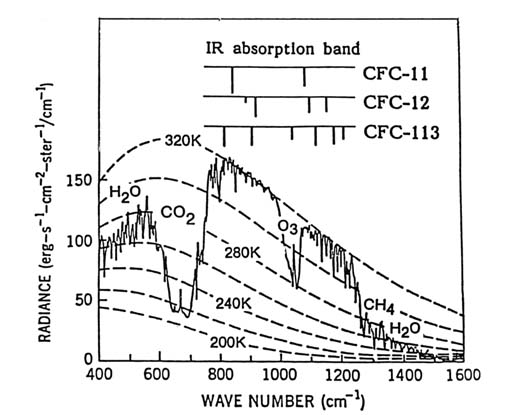
Figure 1. Infrared emissions over Sahara Desert as observed by IRIS-D instrument
on Nimbus-4 satellite. Expected intensities for different temperatures are indicated
by dashed lines. Emissions direct from surface (at 320° K or 117° F) are observed in
"transparent" regions between 800–1000 cm^-1 and 1100–1250 cm^-1 ; strong absorption
regions for CO₂ , O₃ , H₂ O, and CH₄ are indicated. The main absorption positions for the
three CFCs are indicated above and are mostly in the transparent regions—making
incremental additions of CFCs far more efficient per molecule in retaining terrestrial
infrared emissions than CO₂ , O₃ , or CH₄ .

(or 54° to 72° F) to force the radiation out through the transparent wavelength windows in the atmosphere and maintain an energy balance with the incoming solar energy.

The existence of transparent and opaque bands in the atmosphere is a well-established fact, already clearly demonstrated by satellite data two decades ago. Figure 1 shows the infrared spectrum escaping from the Earth as seen by the nadir observations of the Nimbus-3 satellite over the Sahara Desert in the year 1970. The surface temperature of the desert was approximately 320° K (117° F), and the upper dashed curve

---

shows the emission intensity expected if all of this IR were able to pass upward directly into space with no atmospheric absorption. For some wavelength regions, the Earth is essentially transparent, and the observed emissions match the 320° K curve expected for the hot desert sands. For other wavelengths, however, the emissions are greatly reduced below the 320° K line because of absorption by CO₂ , O₃ , and H₂ O as marked. Already twenty years ago and presumably for eons before, Earth exhibited some regions of unimpeded emission, and others of heavy absorption, consistent with the 34° K temperature increase calculated as the greenhouse effect in the Earth's atmosphere. In other spectra taken from the same satellite, the Pacific Ocean at midnight exhibits in the transparent regions the surface temperature of the nighttime equatorial Pacific, approximately 300° K, and the familiar heavy absorption by carbon dioxide, ozone, and water.

The existence of this natural greenhouse effect is therefore both well understood and experimentally verified by global satellite observations. Our primary current question is this: Is mankind putting into the atmosphere enough additional molecules of CO₂ , H₂ O, O₃ , or other IR-absorbing molecules to increase significantly the ability of the atmosphere to hold in IR radiation? If so, then the terrestrial response to lessened IR escape at those wavelengths will simply be to raise the temperature of the Earth to push a little bit more out through the transparent windows. This extra warming will force still more IR radiation out through the transparent regions—instead of a 34° warming from the greenhouse, an average of 36° or 38° may be required. Because we have experienced the adjustment of 30°–40° warming for thousands of years we think of it (correctly) as normal and speak of the greenhouse effect in 1989 in terms of the prospective increment of another 2° or 4° above the long-term base. The suggestion that the CO₂ released by the burning of carbonaceous fossil fuels such as oil, coal, and natural gas might cause such an elevation of the greenhouse temperature had already been made in the 1890s and was raised again more urgently in the 1950s and 1960s. The worldwide growth in atmospheric CO₂ was established in the 1960s through the measurements of Professor C. D. Keeling of the Scripps Institution of Oceanography. His measurements continue, as shown in figure 2.

A very important factor in the scientific evaluation of "greenhouse warming" during the last decade has been the realization that this is not just a problem of increasing CO₂ but is rather a more general problem of increasing concentrations of many trace gases. Atmospheric measurements (fig. 2) have clearly shown a CO₂ increase of about 12 percent since 1958, from 315 parts per million by volume (ppmv) in 1958 to 355 ppmv in 1989. In the mid-1970s, the chlorofluorocarbon (CFC) gases such as CCl₃ F and CCl₂ F₂ were shown first to be accumulating in the

---

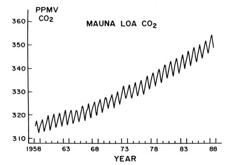
Figure 2. Carbon dioxide concentrations in parts per million by volume as measured at
Mauna Loa, Hawaii, by C. D. Keeling of Scripps Institution of Oceanography.

atmosphere and then to be important as greenhouse gases. Early in the 1980s, methane (CH₄ ), as shown in figure 3, and nitrous oxide (N₂ O) were also proven to be increasing their atmospheric concentrations.

The observed increase rates for several trace gases are given in table 1, expressed in parts per trillion (10¹² ) by volume (pptv). In these units, the carbon dioxide concentration in the 1989 atmosphere is about 355,000,000 pptv, and the yearly rate of increase is about 1,500,000 pptv. This absolute rate of increase for CO₂ in pptv/year is very much larger than for any other atmospheric trace gas. For example, the yearly increase in carbon dioxide is more than a thousand times larger than the total concentration of the chlorofluorocarbons in the atmosphere. Chlorofluorocarbon-12 (CCl₂ F₂ ) is increasing only by 16 or 17 pptv per year with a concentration around 450 pptv in the late 1980s.

How it is that one molecule (CCl₂ F₂ ) increasing at 17 pptv per year can possibly play a significant role in the greenhouse effect, when another (CO₂ ) is going up by 1,500,000 pptv per year, almost 100,000 times faster?

The structure of the CFC molecules is such that their individual molecular vibrations furnish very strong IR absorption at different wavelengths

---

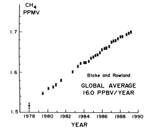
Figure 3. Globally averaged concentrations of methane, as measured in the Pacific
Region between 71°N-47°S latitudes by D. R. Blake and F. S. Rowland.

from CO₂ , H₂ O, and O₃ and fall right in the middle of the transparent wavelength regions, as indicated in figure 1. An additional molecule absorbing in the transparent region is very much more efficient in retaining IR radiation than one additional molecule of CO₂ , because the latter can only absorb the same wavelengths being swallowed up by the 355,000 pptv of CO₂ already present in the atmosphere. In an artificial atmosphere free of both CO₂ and CFCs, individual molecules of CO₂ and CFC are roughly comparable in retaining IR radiation. In Earth's relatively CO₂ -rich atmosphere, however, the addition of more CO₂ is a form of overkill in IR absorption and is not very effective per added molecule , as shown in table 1. Nevertheless, the sheer magnitude of the yearly 1,500,000 pptv increase in CO₂ is enough to retain for carbon dioxide increases the most important role in the greenhouse effect.

As shown in table 1, the chlorofluorocarbons are about 20,000 to 25,000 times as efficient as added carbon dioxide in the 1989 atmosphere.

---

TABLE 1. Contributions to the Greenhouse Effect from Concentration Changes in Atmospheric Trace Gases

Methane is about 30 times as efficient as CO₂ in the Earth's atmosphere. These high relative efficiencies, taken with the known concentration increases, cumulatively have greenhouse impacts that begin to match that of carbon dioxide.

How sure are scientists that these trace gases are increasing in average global concentration? This is a question for which some of the answers have been provided by the trace gas measurements performed by my own research group. Our involvement in atmospheric chemistry started with the observations in 1971 by James Lovelock that the molecule tri-chlorofluoromethane (CCl₃ F) was present at a level of about 60 or 80 pptv in the north temperate zone and about 40 pptv south of the equator. Contemplation of these findings led to scientific curiosity and eventually the questions: What will happen to the CFC molecules in the atmosphere? How long will it take?

The answer to the first question is now often called the Rowland-Molina theory of stratospheric ozone depletion by chlorofluorocarbons. The CFCs eventually are blown apart by solar UV in the mid–stratosphere, releasing atomic Cl, which then proceeds to destroy globally significant amounts of ozone by a chain reaction process. The full scientific description of ozone depletion is a separate topic and has been discussed extensively elsewhere.

The important aspect of the Rowland-Molina theory as far as the greenhouse effect is concerned is contained in the answer to the "how long" question: the CFCs last many decades. The time scale for the removal of CFC-11 (CCl₃ F) from the atmosphere is about 75 years on the average, while its companion molecule, CFC-12, requires approximately

---

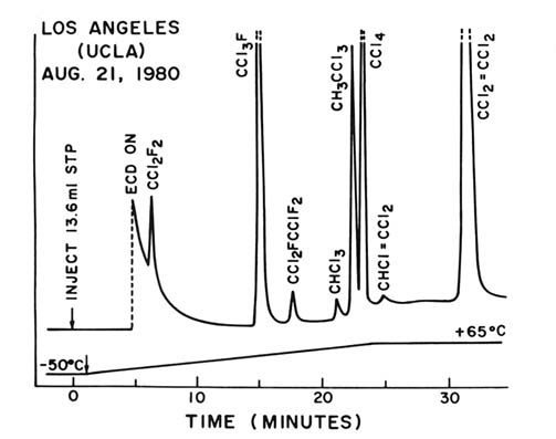
Figure 4. Electron capture gas chromatogram of an air sample collected on the UCLA
campus on August 21, 1980—a typical urban sample. The time on the horizontal axis
serves to identify the individual trace gases present in the sample, and the height on
the vertical axis measures the quantity present. Because the individual molecular sensitivities
are different, the peak heights are separately calibrated. The vertical dashed lines indicate
off-scale peaks.

120 to 140 years. While such long lifetimes were originally estimated theoretically by Rowland and Molina, they have now been confirmed by actual measurements in the atmosphere itself. From the differences between the total amounts released and still present in the atmosphere, now measured over a time period of more than 15 years, the atmospheric lifetimes have been established to be fully as long as originally calculated.

Figure 4 shows a "gas chromatogram" of air taken from the UCLA campus in Los Angeles in 1980. The chemical identity of different compounds is established by the distance along the horizontal time axis: each molecule has its own characteristic travel time through the sixty-meter-long gas chromatographic column. The atmospheric concentration of each compound is shown by the vertical height of its corresponding

---

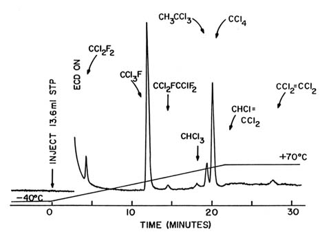
Figure 5. Electron capture gas chromatogram of an air sample collected at Nosappu Point
on the Japanese island of Hokkaido on August 3, 1979—a typical remote-location
sample. The vertical scale is the same as in figure 4.

peak. (Because the instrument sensitivity varies widely with different compounds, each peak height requires its own calibrated scale for conversion into pptv units.) Three successive CFC peaks—CFC-12, CFC-11, CFC-113 (CCl₂ FCClF₂ )—are followed by chloroform (CHCl₃ ), methyl chloroform (CH₃ CCl₃ ), carbon tetrachloride (CCl₄ ), trichloroethylene (CHCl=CCl₂ ), and tetrachloroethylene (CCl₂ =CCl₂ ). These peaks are quite representative of the usual composition of air in urban environments—the standard loading found in cities into whose atmosphere a lot of chlorinated molecules are being released. A similar 1980 air sample taken in San Jose, California, showed the same eight molecules, albeit with much more CFC-113, because this molecule was already then widely used for cleaning electronics. The large CFC-113 peak was a characteristic of San Jose air—a trademark for Silicon Valley and its electronic industries—and is even more prominent in 1989.

However, the global concentration of these molecules cannot be estimated from such data taken in the cities, which are the major sources for the man-made CFCs. Rather, extensive sets of observations must be made in remote locations. Figure 5 shows the concentration data from the easternmost tip of the island of Hokkaido in Japan, a very remote

---

location. Seven of the same eight compounds are present, but in much smaller concentrations. The concentration of CHCl=CCl₂ is almost undetectable, because it has a survival time in the atmosphere of only a few weeks, and the Hokkaido air had traveled for many weeks without passing over a major city.

For eleven years I and the members of my research group have been traveling regularly to remote locations from Alaska to the South Pole, bringing back air samples for trace gas analysis. Our data and those of several other research groups have clearly shown rapid worldwide increases in the concentrations of each of the CFCs. The growth in the organochlorine concentrations in the atmosphere is graphed in figure 6, with actual data back to 1971. Extrapolations farther backward in time are based on known production figures, while forward estimates are based on various hypotheses for future global emission trends.

Methyl chloride, CH₃ Cl, is the only molecule shown in figure 6 for which an important known natural source exists. (Kelp beds produce the related compound methyl iodide, CH₃ I. As methyl iodide percolates up through seawater, chloride ion displaces the iodine, forming CH₃ Cl.) As far as we can determine, the 600 pptv concentration of CH₃ Cl is almost entirely natural, and the measured values have not changed during more than a decade of observations. In contrast, CCl₄ , CFC-11, CFC-12, CFC-113, and CH₃ CCl₃ have been steadily adding to the total chlorine loading of the atmosphere. Whereas the atmosphere is assumed to have contained about 0.6 parts per billion by volume (ppbv) in 1900 (essentially only CH₃ Cl), the total chlorine loading was about 0.8 ppbv in 1950, 1 ppbv about 1965, 2 ppbv around 1976, and is now approximately 3.5 ppbv in 1989. Worldwide, there has been a very substantial increase in the total amount of atmospheric chlorine, and most of this increase has been accounted for by the growth of these long-lived CFC compounds.

Each of these three CFC gases absorbs strongly in the transparent region of the infrared. As shown in table 1, the CFCs together make an atmospheric greenhouse contribution that significantly adds to that of carbon dioxide. If we were to continue putting these molecules into the atmosphere at the rate we were doing in 1986, then the concentrations will rise as shown by the thin solid lines in figure 6, with a total atmospheric chlorine concentration reaching 5 ppbv early in the next century. The provisions of the United Nations Montreal Protocol, agreed to by all of the major nations in September 1987, took effect in July 1989 and call initially for a cutback in CFC emissions to the 1986 levels. The Montreal Protocol then requires a 20 percent cutback from the 1986 levels in 1994, and a 30 percent additional cutback in 1999. These reductions would produce the chlorine concentrations shown by the dotted lines (fig. 6). The Protocol as now established does not really make

---

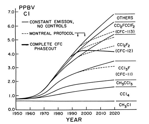
Figure 6. Averaged Northern Hemispheric chlorocarbon concentrations in the atmosphere
at surface level. Actual measurements from early 1970s to the present. Extrapolated back
to 1950 from known production figures. Extrapolated forward to 2020 with several different
assumptions: (a) continued yearly emissions at 1986 levels (thin solid lines); (b) yearly
emissions modified according to Montreal Protocol of September 1987—reduction to
80 percent of 1986 levels in 1994, and to 50 percent of 1986 levels (dashed lines); and
(c) complete phaseout of CFC emissions by the year 2000 (thick solid line).

much difference until the next century, and total chlorine would still rise rapidly, although not as rapidly as without it.

The terms of the Montreal Protocol are in the process of being greatly strengthened. For instance, the European Economic Community announced in March 1989 that its twelve countries will no longer be emitting chlorofluorocarbons by the end of the century. The major U.S. manufacturers of CFCs such as DuPont and Allied-Signal have also said that they will phase out the production of chlorofluorocarbons by the end of the century. If these actions are carried through as planned, much of the problem of the growth in CFCs will be taken care of within

---

the next decade or so. The growth of total atmospheric chlorine concentration should peak between 4.0 and 4.5 ppbv at the end of the decade, and then gradually decrease. Even with the total phaseout of CFC production, however, the chlorine concentrations will remain high for all of the twenty-first century. The slow decrease as shown by the thick solid line in figure 6 is the straightforward result of the long atmospheric lifetimes of the CFCs.

In 1978 we made our initial measurements of the concentrations of methane in the atmosphere. At that time the concentration in the Northern Hemisphere was about 1.58 ppmv and in the Southern Hemisphere about 1.46 ppmv, for a global average of 1.52 ppmv. Our repeated measurements since then have shown a steady, parallel increase in both hemispheres to a 1989 global average of 1.70 ppmv, as shown in figure 3. We now make these measurements every three months, going everywhere from Alaska to New Zealand, with visits to the South Pole in the summer, bringing back air samples from which we derive a global average.

Our data show an average increase in methane of 16 ppbv/year over the time period of eleven years, a 12 percent increase. The atmosphere is certainly increasing its concentration of methane, bringing with it the ability to absorb infrared radiation in wavelengths that are different from those of carbon dioxide. The CH₄ contribution to greenhouse warming also adds significantly to that from CO₂ , and, unlike the CFCs, controls will be much harder to apply.

The sources of methane in the atmosphere are roughly 75 percent biological—from microbial action in swamps, rice paddies, cattle stomachs, and so on—and perhaps 25 percent from methane released in the production and use of fossil fuels. We know rather accurately that the atmospheric lifetime of methane is about ten years, which means that 10 percent of the 4,800 megatons in the atmosphere must be replaced each year. While we know that about 500 megatons of CH₄ is released each year, assessment of the distribution among those contributors is more difficult. However, it is possible to distinguish biological methane from fossil-fuel methane, because biological methane has carbon-14 in it and fossil-fuel methane does not. Carbon-14 atoms are formed continually in the atmosphere by nuclear reactions induced by high-energy cosmic radiation and become incorporated first into ¹⁴ CO₂ and then by photosynthesis into plants and ultimately into all living species. Because ¹⁴ C is radioactive with a half-life of 5,700 years, the carbon residues of biological species remain radioactive for periods of tens of thousands of years. Coal, oil, and natural gas, however, have been sequestered from cosmic radiation for millions of years and no longer have any ¹⁴ C. The measurements of the ¹⁴ C content of atmospheric methane lead to the interpretation that about 75 percent is biological and the rest of it probably

---

originates from fossil fuel. (These measurements are made less precise by the "pulse" of ¹⁴ C introduced into the Earth's atmosphere by the testing of nuclear weapons in the atmosphere during the 1950s and early 1960s.)

Measurements of the atmospheric concentrations of CO₂ and CH₄ can now be carried out for thousands of years into the past. The major route to this information about earlier atmospheric composition is from ice cores taken out of the accumulated layers of ice lying over a bedrock base in Greenland and Antarctica. At the Vostok station operated in Antarctica by the Soviet Union, the buildings lie about 4,000 meters above the solid bedrock with intervening layers of 4,000 meters of ice gathered year by year above the rock. Vostok is necessarily at high altitude and is very cold (an average temperature of about — 59° F), with only a little snowfall each year. The Vostok ice sheets have been cored down 2,200 meters, which corresponds to an ice accumulation for 160,000 years, with little bubbles of air trapped all along the way. The present warm period (the Holocene) began about 20,000 years ago, preceded by an icy period of about 100,000 years, then another warm or interglacial period, and then another time of ice. A core going back 160,000 years extends through the most recent series of ice ages, beyond the last interglacial period, and into another earlier sequence of ice ages. Swiss and French scientists have measured the concentrations of CO₂ and CH₄ throughout this long period.

The concentration of CH₄ was no larger than 0.7 ppmv during our present warm period until the last 200 years or so, and was also about 0.6–0.7 ppmv during the last interglacial 130,000 years ago. In between, during the fluctuations of most recent ice ages, the CH₄ concentrations varied from 0.3 to 0.4 ppmv; the level was also 0.3 to 0.4 ppmv in the ice age 150,000 years ago. Over all the past 160,000 years, except the last 200, the CH₄ concentration varied from 0.3 to 0.7 ppmv through ice ages and interglacials. Changes of 0.3 ppmv in CH₄ concentration took place over millennia, varying between 0.3 and 0.7 ppmv. By comparison, when we started our measurements in 1978, the concentration was 1.52 ppmv and now, in 1989, 1.70 ppmv, and increasing 0.1 ppmv every 6 years. We are truly moving rapidly into previously uncharted areas.

The most famous series of trace gas measurements is shown in figure 2, with the CO₂ measurement made on top of Mauna Loa, Hawaii, by C. D. Keeling. The pattern shows the annual "breathing" of the Northern Hemisphere, with rapid CO₂ decreases as it is used in photo-synthesis by the green plants in spring and summer together with the year-round release of CO₂ from the decay of biological material. This annual cycle is superimposed on a steadily rising background, so that the yearly average CO₂ concentration has increased about 12 percent from 315 to 355 ppmv in 31 years.

---

In summary, the CFCs are increasing at 5 percent per year with CFC-113 going up at a more rapid rate; methane approximately 1 percent per year; CO₂ by 0.5 percent per year; N₂ O about 0.2 percent per year. These rates of increase have been fed into detailed models of the infrared absorbing characteristics of the atmosphere, and have provided the estimated relative contributions from the various trace gases as summarized in table 1.

Most such calculations were carried out before the intense concerns in the past two years over ozone depletion by CFCs. The future estimates of the CFC influences will no longer show the incremental IR contributions characteristic of the 1980s. By the year 2000, CFC emissions are likely to be nearly zero, except for residual release from existing equipment. This part of the greenhouse problem has apparently been solved on an international basis, although the rapidity of implementation of the solution over the next decade will still have important atmospheric consequences. The concern over stratospheric ozone depletion by the CFCs stopped the exponential growth in CFC production in the mid-1970s, converting it into more or less constant release for a decade before growth began in the mid-1980s. Without the restrictions and doubts placed upon CFC growth in the 1970s, the greenhouse problem in the 1990s would have been a CFC problem augmented by CO₂ , rather than a CO₂ problem augmented by CFCs and other trace gases. However, nitrous oxide and methane emissions have not been curtailed or even well understood, and their concentrations will continue to grow.

Carbon dioxide is still the major contributor to the greenhouse effect, and its yearly contribution appears to be increasing. Figure 2 shows that the amount of carbon dioxide over Hawaii begins to decrease in March or April because of the seasonal growing cycle in the Northern Hemisphere. Throughout the year the continuing decomposition of plants releases CO₂ , and the burning of fossil fuels releases CO₂ , and these increases are not countered by photosynthesis during the late autumn and winter. Each year the spring value is a little bit higher than the year before. The magnitude of the seasonal cycle is slowly increasing from about 7 ppmv in the 1960s to 8 ppmv in the 1980s. The change is not large, but the breathing cycle is expanding.

However, after allowing for the seasonal cycle, the growth from 315 ppmv to around 355 ppmv has been very steady, although not uniform. In the 1960s the yearly increase was about 0.8 ppmv/year; in the 1980s, about 1.5 ppmv/year. In the last two or three years, the increase has been more than 2 ppmv/year. The implication is strong that the growth in CO₂ underlying the greenhouse effect is accelerating.

An important question for dealing with the greenhouse effect will be the full understanding of these CO₂ concentration changes. The total amount of carbon from the burning of fossil fuel that is going into the

---

atmosphere is considerably larger than the carbon dioxide increase registered in the atmosphere. This discrepancy is described by the concept of an "airborne fraction," i.e., the fraction of CO₂ that hasn't disappeared from the atmosphere by going into the ocean or some other place. The airborne fraction was about 50 percent in the 1960s but is now approximately 60 percent. Appreciable CO₂ contributions are also being received from the burning of the tropical forests. It is important that we understand all the characteristics of this curve in order to understand how to predict and control future carbon dioxide concentrations in the atmosphere. Similarly, it will be important to understand the individual contributions from various processes toward methane and nitrous oxide emissions.

The procedures necessary to solve the chlorofluorocarbon problem have been put into place on an international scale and have begun to be implemented. We still have left for the future, however, efforts to reduce emissions of carbon dioxide, methane, and nitrous oxide. The advantages of prevention over cure in the realm of atmospheric problems are illustrated by the time scale for atmospheric recovery from the CFC releases of the past two decades. Stratospheric ozone depletion and infrared greenhouse absorption will be caused by the chlorofluorocarbons in the atmosphere for all of the twenty-first century, because the lifetime of these molecules is very long. A return to the stratospheric chlorine concentrations of the 1960s will not happen before the twenty-third century.

Appendix

---

---

---

---